Estimate Direction of Arrival Using MUSIC Algorithm and TwinRX Daughterboards
This example shows how to estimate the direction of arrival of a signal with a multiple signal classification (MUSIC) algorithm using a USRP™ X310 radio with TwinRX daughterboards.
Required Hardware
To run this example, you require:
A USRP X310 radio with two TwinRX daughterboards. You can also convert an equivalent National Instruments radio (NI-2945R or NI-2955R).
A second USRP radio to transmit a stimulus signal.
Five antennas.
Four SMA cables of equal length.
For more information about which USRP radios are supported in Wireless Testbench™ and how to convert a NI-2945R or NI-2955R radio to a USRP X310 radio, see Supported Radio Devices.
Introduction
Direction of arrival (DOA) estimation involves determining the direction from which a received signal originates relative to a receiver antenna array. This process has applications in tracking moving objects, localizing signal sources, and beamforming.
The MUSIC algorithm is a high-resolution DOA estimation algorithm based on the eigenvalue decomposition of the sensor covariance matrix observed at an array. This algorithm exploits the orthogonality between the signal subspace and the noise subspace to determine the DOA. For more information, see MUSIC Super-Resolution DOA Estimation (Phased Array System Toolbox).
In this example, you:
Set up your USRP X310 radio with TwinRX daughterboards to have four phase-synchronized receive channels connected to linear array of antennas.
Use a second USRP radio to transmit a 10 kHz signal.
Capture and process the received signal using the MUSIC algorithm to estimate the angle of arrival, which you visualize using an app.
The direction of arrival estimation uses the phased.MUSICEstimator (Phased Array System Toolbox) System object™, which implements the spatial spectrum of the incoming signal by using a narrowband MUSIC beamformer for a uniform linear array (ULA).
The diagram shows an overview of the example.
Connect and Set Up Hardware
Before you run this example, follow these steps:
Set up your USRP X310 radio with TwinRX daughterboards for companion LO sharing. For details, see LO Sharing Using USRP X300/X310 with TwinRX Daughterboards.
Use the Radio Setup wizard to connect and set up both USRP radios.
Set up a linear array of four antennas with a distance between antennas equal to the wavelength of the transmitted signal divided by two. The example uses a center frequency of 2.4 GHz, which corresponds to a spacing of 6.25 cm between each antenna. Connect all four receiver channels of the USRP X310 radio to the antennas in the antenna array from left to right to provide the correct orientation for the display.
Set Up Radio
Call the radioConfigurations function. The function returns all available radio setup configurations that you saved using the Radio Setup wizard.
savedRadioConfigurations = radioConfigurations;
To update the dropdown menu with your saved radio setup configuration names, click Update. Then, use the radioConfigurations function to create a radio object for each of the two radios you select to use with this example.
savedRadioConfigurationNames = [string({savedRadioConfigurations.Name})];
 receiveRadio = radioConfigurations(
 savedRadioConfigurationNames(1));
transmitRadio = radioConfigurations(
savedRadioConfigurationNames(1));
transmitRadio = radioConfigurations( savedRadioConfigurationNames(2));
Configure Transmitter
Create a basebandTransceiver application object to act as the transmitter. Set the sample rate to 1 MHz, the center frequency to 2.4 GHz, and the gain to an appropriate value for your radio.
sampleRate =1000000; centerFrequency =
2400000000; gain =
40; if ~exist('transmitter','var') transmitter = basebandTransceiver(transmitRadio, ... SampleRate=sampleRate, ... TransmitRadioGain=gain, ... TransmitCenterFrequency=centerFrequency); end
Transmit Source Signal
First, transmit a signal for calibration. Create a dsp.SineWave System object to generate a 10 kHz tone. For calibration, place the transmit antenna centered in front of the receiver antenna array at an elevation close to zero.
transmitToneFrequency =10000; transmitToneAmplitude =
1; sineSource = dsp.SineWave (... 'Frequency',transmitToneFrequency, ... 'Amplitude',transmitToneAmplitude,... 'ComplexOutput',true, ... 'SampleRate',sampleRate, ... 'SamplesPerFrame',round(transmitter.SampleRate/transmitToneFrequency), ... 'OutputDataType','double'); sourceSignal = sineSource();
Transmit the tone continuously.
transmit(transmitter,sourceSignal,'continuous');Configure Receiver
Create a second basebandTransceiver application object to act as the receiver. Set the sample rate and center frequency to the same values as the transmitter and set the gain to an appropriate value for your radio. Set the DroppedSamplesAction property to none to suppress warnings when samples are dropped.
if ~exist('receiver','var')
    receiver = basebandTransceiver(receiveRadio,...
        SampleRate=sampleRate,...
        CaptureAntennas=["RFA:TX/RX","RFA:RX2","RFB:TX/RX","RFB:RX2"], ...
        DroppedSamplesAction ='none', ...
        CaptureRadioGain=gain, ...
        CaptureCenterFrequency=centerFrequency, ...
        CaptureDataType='double');
end
Specify a capture length of 4000 samples.
captureLength =  4000;
4000;Set Up Calibration Plots
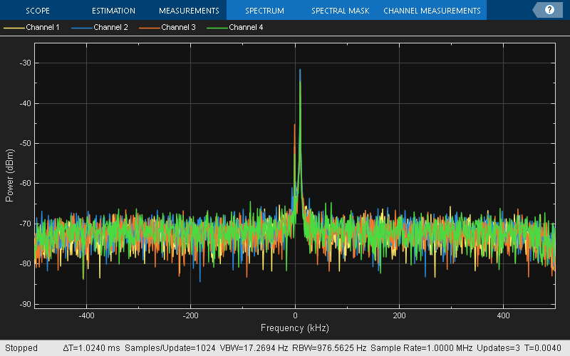
Create a spectrumAnalyzer and timescope System object to visualize the received signal in the frequency and time domains.
spectrumScope = spectrumAnalyzer(SampleRate=sampleRate);
timeScope = timescope(TimeSpan=4/transmitToneFrequency,SampleRate=sampleRate);
Estimate and Correct Phase Offset
Verify that the source signal is being transmitted by capturing samples and visualizing the data using the spectrum analyzer. Set UseRadioBuffer to false to capture data directly to the host, bypassing the onboard radio memory buffer, which is required to capture data from more than two antennas on the USRP X310 radio.
[data, valid, overrun] = capture(receiver,captureLength,UseRadioBuffer=false);
spectrumScope(data);

Use the basebandPhaseAnalyzer object to estimate the phase offset between the four receiver channels.
analyzer = basebandPhaseAnalyzer(RadioApplication=receiver);
[rxPhases,rxResults] = measureAntennaPhase(analyzer,"capture",SamplesPerAntenna=10000);
Set Up Direction of Arrival Estimator
Configure a phased.MUSICEstimator (Phased Array System Toolbox) System object for estimating the direction of arrival of a signal. The sensor array is defined as a ULA with a spacing of lambda/2.
lambda = physconst('LightSpeed')/centerFrequency;
array = phased.ULA(NumElements=4,ElementSpacing=lambda/2);
estimator = phased.MUSICEstimator( ...
    SensorArray=array, ...
    OperatingFrequency=centerFrequency, ...
    ForwardBackwardAveraging=true, ...
    DOAOutputPort=true, ...
    NumSignalsSource='Property', ...
    NumSignals=1, ...
    SpatialSmoothing=1);
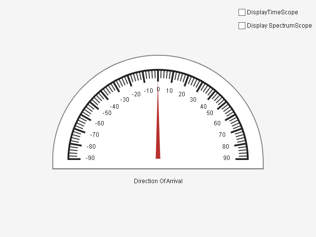
Display Direction of Arrival
Use the wtDOAEstimationApp app to display the direction of arrival of the transmitted signal and to display the time and frequency plots of the received signal. Select Display TimeScope or Display SpectrumScope to monitor power and the frequency of the signal received by the antenna array.
app = [];
if isempty(app)
app = wtDOAEstimationApp();
end
Set the simulation to capture 1000 seconds of data.
stopTime = 1000;
startTime = tic;
Estimate Angle of Arrival
In a loop, capture data, normalize and phase-align the four receive channels, estimate the DOA, and update the app for visualization in real time. The semicircular gauge in the app shows the estimated direction of arrival in degrees. The loop runs until the stop time is reached.
try
    % Loop until the timeCounter reaches the target stop time.

    while (toc(startTime) < stopTime)

        [data, valid, overrun] = capture(receiver, ...
            captureLength,UseRadioBuffer=false);

        if ~overrun

            data = wtDOAEstimationAmplitudeNormalization(data);

            % Rotating IQ data
            data = wtDOAEstimationRotateIQ4Channels(data, ...
                rxPhases{1}(2),rxPhases{1}(3),rxPhases{1}(4));

            % Calculating the direction of arrival
            [~,doas] = estimator(data);

            drawnow limitrate; % Adding pause for UI Update

            % Display angle in UI
            if isscalar(doas)
app.displayAngle(doas);
            end

            % Visualize in time domain
            if(app.DisplayTimeScopeCheckBox.Value)
                timeScope(data);
                dataMaxLimit = max(max(abs([real(data); imag(data)])));
                timeScope.YLimits = [-dataMaxLimit*1.5, dataMaxLimit*1.5];
            end

            % Visualize frequency spectrum
            if(app.DisplaySpectrumScopeCheckBox.Value)
                spectrumScope(data);
            end

        end
    end
catch ME
    release(timeScope);
    release(spectrumScope);
    rethrow(ME);
end

The animated GIF shows an example.
Release the visualization scopes, stop the transmitter, and delete the app handle.
release(timeScope);
release(estimator);
release(spectrumScope);
stopTransmission(transmitter);
delete(app);
Further Exploration
To improve performance of the estimation, you can modify the example to use the phased.RootMUSICEstimator (Phased Array System Toolbox). Additionally, you can synchronize and combine multiple radios to create a larger antenna array.
Troubleshooting
To avoid multi-path reflections, test this example in an open environment. Hold the transmitting and receiving antenna array at the same elevation. If you are working in a closed space, keep the transmitter in the near field of the antenna array.
For proper reception of the signal, you may need to increase the gain of the transmitter after connecting to the antenna array.
The MUSIC algorithm estimates the broadside angle (azimuth angle) only when the elevation angle is near zero. To get an accurate DOA, ensure that the elevation angle is near zero
This example estimates the angle continuously from -70 to 70 degrees. When you move the transmitter beyond these limits, discontinuities appear in the estimated angle.
To increase the accuracy of the estimated DOA, calibrate the antenna array setup with a power splitter and matched cables.
See Also
Functions
Objects
basebandTransceiver|basebandPhaseAnalyzer|phased.MUSICEstimator(Phased Array System Toolbox)