Demonstrate Extremal Phase Property
For a given support, the cumulative sum of the squared coefficients of a scaling filter increases more rapidly for an extremal phase wavelet than other wavelets.
Generate the scaling filter coefficients for the db15 and sym15 wavelets. Both wavelets have support of width .
n = 15;
lor_db = daubfactors(n);
lor_sym = daubfactors(n,"sym");
Next, generate the scaling filter coefficients for the coif5 wavelet. This wavelet also has support of width .
lor_coif = coifwavf("coif5");Confirm that the sum of the coefficients for all three wavelets equals 1.
sum(lor_db)
ans =
1.0000
sum(lor_sym)
ans =
1.0000
sum(lor_coif)
ans =
1.0000
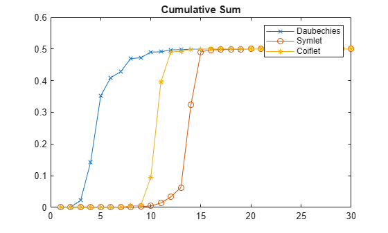
Plot the cumulative sums of the squared coefficients. Note how rapidly the Daubechies sum increases. The sum increases rapidly because its energy is concentrated at small abscissas. Since the Daubechies wavelet has extremal phase, the cumulative sum of its squared coefficients increases more rapidly than the other two wavelets.
plot(cumsum(lor_db.^2),"x-")
hold on
plot(cumsum(lor_sym.^2),"o-")
plot(cumsum(lor_coif.^2),"*-")
hold off
legend("Daubechies","Symlet","Coiflet")
title("Cumulative Sum")