Understanding IBIS-AMI Simulations
IBIS-AMI models represent an alternative to the traditional approach to time-domain simulation. They can simulate a much larger number of bits and verify lower bit error rates. IBIS-AMI approach is based on two fundamental assumptions:
You can break a transmitter or receiver into two independent parts:
an analog part representing the output buffer and termination of the transmitter or an input termination of the receiver, and
an algorithmic or digital part modeling the equalization capabilities of the device.
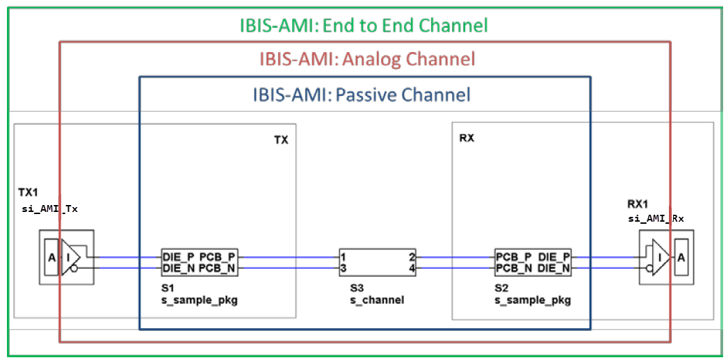
The analog parts of the transmitter, receiver, and the passive interconnects are linear and time-invariant (LTI). This allows you to characterize them completely by a single impulse response. This path from output buffer through the passive interconnect to the input buffer is referred to as the analog channel
Based on these two assumptions, you can create an eye diagram at the receiver in two different ways. Each method implies a different type of algorithmic model.
First, you can create a statistical eye at the receiver if the algorithmic portions of the transmitter (TX) and receiver (RX) are LTI and you can model them with an impulse response. The statistical simulation has no bit stream. Instead, it constructs an eye showing all combinations of bits capable of generating inter-symbol interference (ISI). The eye is constructed based solely on the impulse response of the channel and the principle of superposition. The eye represents the probability of the signal occurring throughout the unit interval (UI).
You can also generate an eye diagram based on bit-by-bit time-domain simulation. Here, the models for algorithmic portions of the transmitter and receiver can be non-LTI. The models are provided with a bit stream by the electronic design automation (EDA) tool. The bit stream is modified according to the equalization capabilities of the model(s) before being returned to the EDA tool. The eye diagram is constructed by simply overlaying the individual bits. Since the time-domain simulation is carried out on an actual bit stream, you can also model other device features not related to equalization. For example, you can model the clock recovery and adaptive selection of the tap weights of a decision feedback equalizer.
Often, TX or RX models lack the necessary support for the bit-by-bit simulation. However, the EDA tool can use the impulse response of the model in a time-domain simulation through convolution of the impulse response with an input bit stream. This type of simulation is referred to as Init-based time-domain simulation. For more information, see Statistical Analysis in SerDes Systems (SerDes Toolbox).
IBIS-AMI Models
According to the IBIS-AMI specification, SerDes executable transmitter or receiver models can contain up to three functions:
AMI_Init, required functionAMI_GetWave, optional functionAMI_Close, required function
All equalization or clock recovery capabilities are modeled in the
AMI_Init and AMI_GetWave functions. If you want
to use the model for statistical simulations, AMI_Init accepts an input
impulse response from the EDA tool, convolves it with the impulse response of the device,
and returns the result. If you want to use the model for time-domain simulations,
AMI_GetWave accepts an input bit stream, modifies it based on the
equalization features of the device, and returns the modified bit stream to the EDA tool.
You need an EDA tool to call the AMI_Init function of a model
regardless of the type of simulation.
In order to convey the capabilities of a model to an EDA tool, the AMI specification defines two required boolean parameters:
Init_Returns_Impulse — notifies the EDA tool whether the model supports the statistical flow.
GetWave_Exists — indicates whether or not the AMI_GetWave function is available for time-domain simulations.
These parameters are included in the AMI file of the model. All AMI models can be classified as one of three types and the processing flow in a simulation is determined by the particular combination of TX and RX models.
| Model Type | Init_Returns_Impulse | GetWave_Exists | Simulation Capabilities |
|---|---|---|---|
| Init-Only | True | False | Statistical, Init-based time-domain |
| GetWave-Only | False | True | GetWave-based time-domain |
| Dual | True | True | Statistical, GetWave-based time-domain |
Simulation Flow
The TX and RX models are completely independent. For example, if the TX model is of the Init-Only type, there is no requirement that the RX model also be Init-Only. The EDA tool must support all combinations of model types. There are nine possible combination of model types in a single link. The keywords used in simulation flow are:
| Keyword | Definition | Description |
|---|---|---|
| hAC(t) | Impulse response of analog channel. | Product of the network characterization phase of a simulation. Network characterization is required for both statistical and time-domain simulations. |
| hTE(t) | Impulse response of TX equalization. | LTI forms of TX equalizations. |
| hRE(t) | Impulse response of RX equalization. | LTI forms of RX equalizations. |
| gTE[t] | GetWave-based TX equalization. | Time-domain, possibly non-LTI, representations of TX equalizations. |
| gRE[t] | GetWave-based RX equalization. | Time-domain, possibly non-LTI, representations of RX equalizations. |
Tx Init-Only and Rx Init-Only
Neither model has an AMI_GetWave function. So you can only
perform statistical or Init-based time-domain simulations. The final eye diagrams from the
two flows should be fairly similar since both are using the same, static equalization. Any
difference is due to the finite number of bits in a time-domain simulation. A statistical
eye shows all combinations of bits capable of causing ISI and, as a result, is often
smaller than the time-domain eye.
Tx Init-Only and Rx GetWave-Only
The AMI_Init function of the RX model does not return an impulse
response. So a statistical simulation only includes the TX model and the analog channel.
This means that the final eye diagram is that of the signal at the output of the analog
portion of the RX model which is often the die pad of the receiver device. In a
time-domain simulation, an EDA tool must use the impulse response of the TX model so a
time-domain eye includes the static TX equalization and the dynamic effect of the RX
equalization.

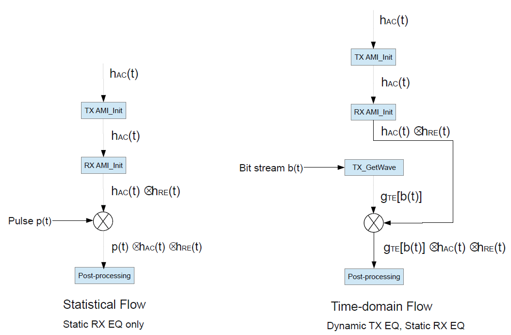
Tx Init-Only and Rx Dual
You can perform a statistical simulation of the entire path. An EDA tool must use the impulse response of the TX model in a time-domain simulation.
The EDA tool is required to call the RX AMI_Init function, which
returns an impulse response reflecting the RX equalization. The equalization is applied
again by the AMI_GetWave function. So, the EDA tool must ensure that
the RX equalization is not applied twice in a time-domain simulation.
This combination of models offers almost a full-featured statistical and time-domain simulations. The only limitation of the flow is the lack of the TX GetWave function and the ability to model dynamic TX equalization. However, TX equalization is generally static and you can choose between statistical and time-domain flows based on the goal of the simulation.
Tx GetWave-Only and Rx Init-Only
The AMI_Init function of the TX does not return an impulse
response. As such, a statistical simulation shows only the effect of the analog channel
and RX model. An EDA tool must use the impulse response of an RX model in a time-domain
simulation.
Tx GetWave-Only and Rx GetWave-Only
Both TX and RX models provide AMI_GetWave functions, so you can
perform full GetWave-based time-domain simulations. However,
Init_Returns_Impulse is false for both models. As a result, a
statistical simulation includes the analog channel characteristics only.
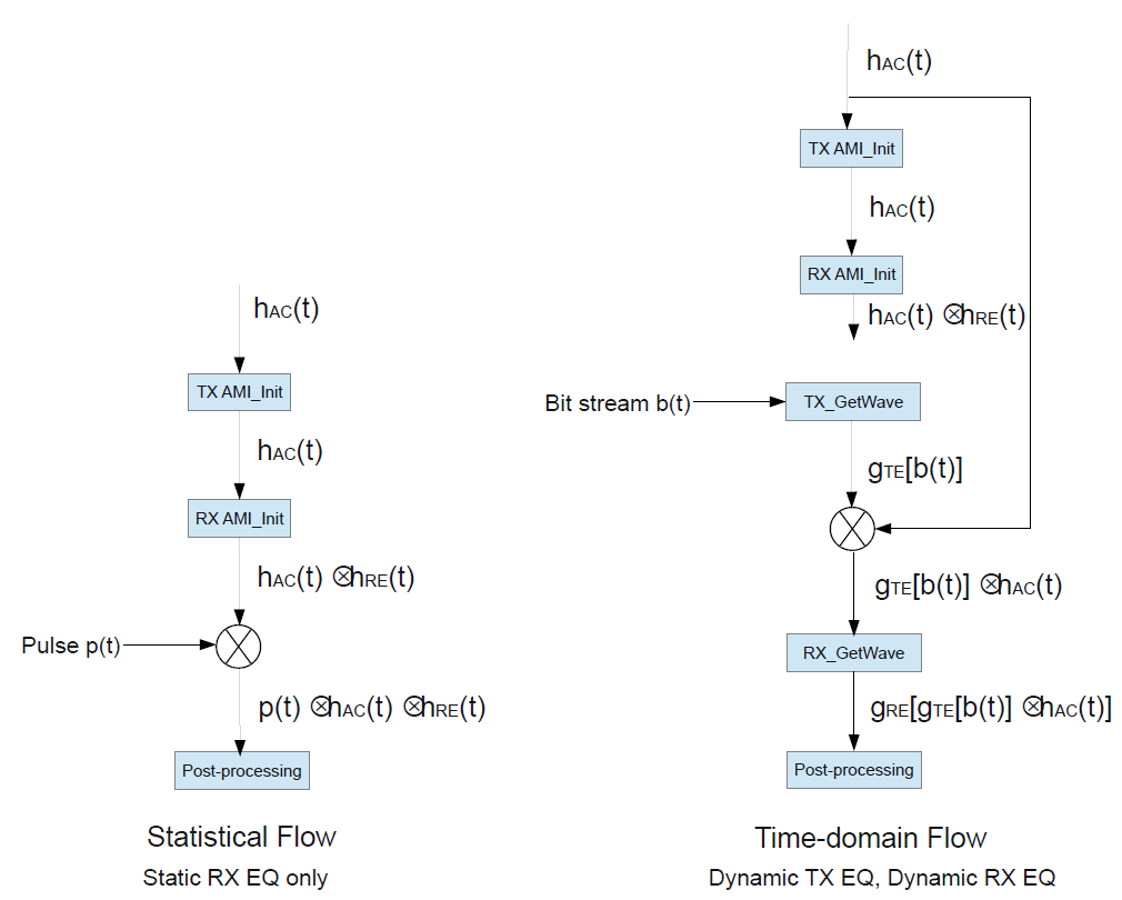
Tx GetWave-Only and Rx Dual
Both TX and RX models provide AMI_GetWave functions, so you can
perform full GetWave-based time-domain simulations. However, the EDA tool must ensure that
the RX equalization is only applied by the AMI_GetWave function.
Init_Returns_Impulse is false for the TX model. As a result, a
statistical simulation includes only the analog channel and RX equalization.
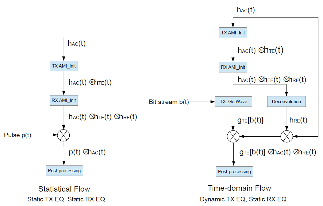
Tx Dual and Rx Init-Only
Init_Returns_Impulse is true for both TX and RX models. So you can
perform a full statistical simulation. The RX model does not include an
AMI_GetWave function so the impulse response must be used in a
time-domain simulation. The EDA tool must ensure that the TX equalization is only applied
by the AMI_GetWave function.
This can present a problem in certain circumstances. For example, as the AMI
specification notes, an RX AMI_Init function may include an
optimization algorithm. In this case, the impulse response presented to the RX
AMI_Init function must include the TX equalization. However, this
leads to a double-counting of the TX equalization in a time-domain simulation.
A possible solution to this problem is an extra processing step involving deconvolution to obtain the impulse response of the RX equalization in isolation. This is then convolved with the impulse response of the active channel and the result is used in a standard GetWave-based simulation. If you are using an EDA tool, you should be aware that deconvolution tends to be numerically ill-behaved. You must exercise caution if the EDA tool implements this extra step.
Tx Dual and Rx GetWave-Only
Init_Returns_Impulse is false for the RX model. So a statistical
simulation only shows the effects of the TX equalization and the active channel. This
means that the final eye diagram is essentially that of the analog portion of the RX model
with no RX equalization. GetWave_Exists is true for both models, so you
can perform a full time-domain simulation. The EDA tool must ensure that the Init-based TX
equalization is not applied in addition to that of the GetWave function.
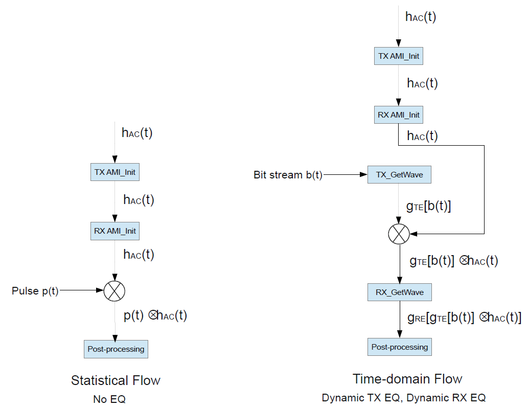
Tx Dual and Rx Dual
Both TX and RX models are capable of statistical and time-domain simulations and you can select either with no limitations. This is the best possible case and the choice between statistical or time-domain flow depends on the goal of the simulation. The EDA tool must ensure there is no double-counting of equalization during a time-domain simulation.
Simulation Flow Summary
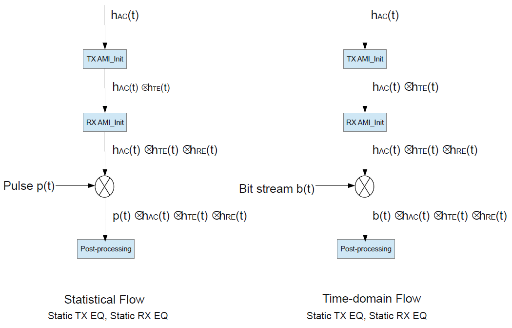
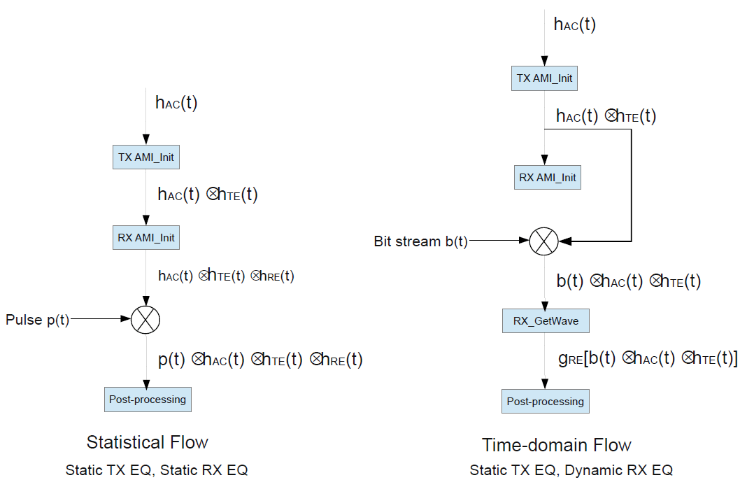
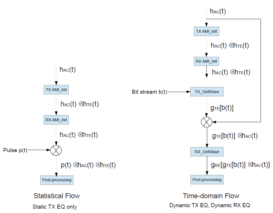
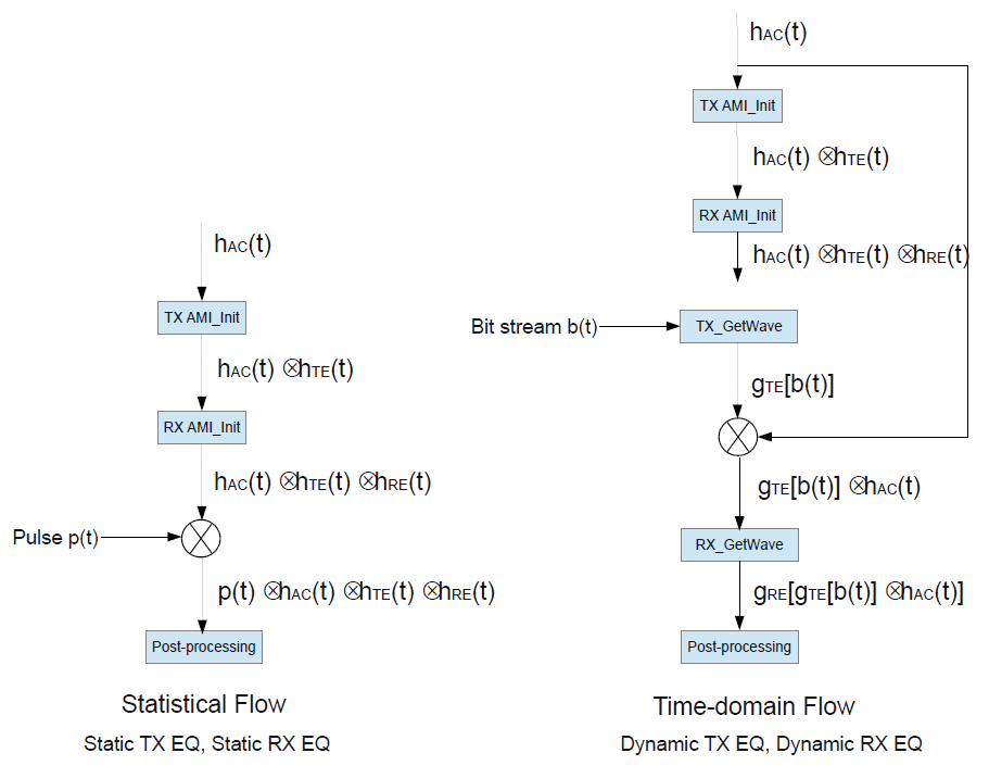
The main elements of the nine different flows can be consolidated into the single diagram:
The statistical flow consists of convolution of the impulse response of the analog channel with the impulse response of the TX equalization, if included in the model, and then convolution with the impulse response of the RX equalization, if included in the model.
The time-domain flow consists of application of the TX
AMI_GetWave function, if it exists, followed by a convolution step,
followed by application of the RX AMI_GetWave function, if it
exists.
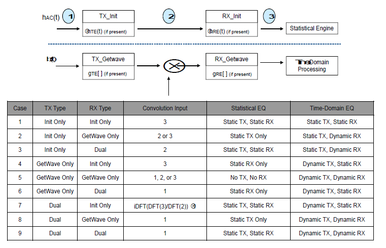
The impulse response used in the convolution step depends on the particular combination of TX and RX models. For example, in a time-domain simulation of Case 2, the impulse response corresponding to steps 2 or 3 of the statistical flow is used to represent the TX equalization.
Case 7 shows one implementation of the extra step required for deconvolution where the Discrete Fourier Transform (DFT) of the impulse response from step 3 of the statistical flow is divided by the DFT of the impulse response from step 2 to give the DFT of the RX equalization only. An inverse DFT transforms the frequency-domain representation of the equalization to an impulse response in the time-domain, to be convolved with the impulse response of the analog channel. This approach is based on the principle that deconvolution in the time domain is equivalent to division in the frequency domain.
Simulation Results in Signal Integrity Toolbox
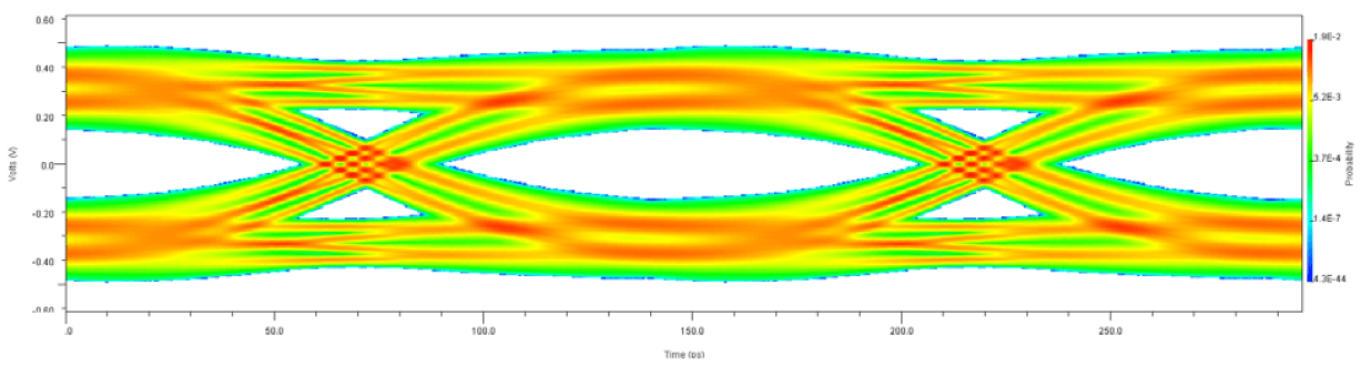
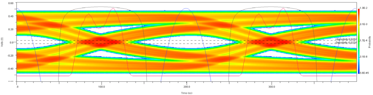
The final result of either a statistical or time-domain simulation is an eye diagram. The eye diagram is then used to generate other common means of evaluating a high-speed channel, in particular bathtub curves and a bit-error-rate (BER). You can also incorporate jitter and noise in a simulation.
Bathtub Curves and BER
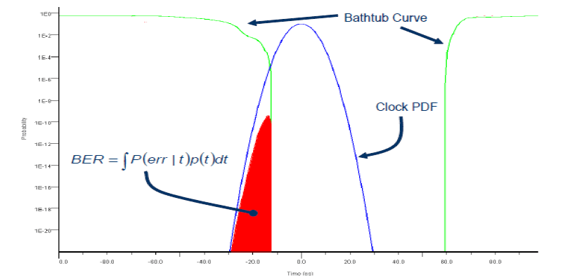
Consider a typical eye diagram along with the probability distribution function (PDF) of the RX clock in blue and the bathtub curve in black. The red trace is the PDF of the time at which the edge crosses the RX threshold. The eye diagram and possibly the RX recovered clock PDF are the direct results of a simulation while the bathtub curve and final BER are calculated in a post-processing step.
In a statistical flow, a user or model must explicitly specify the characteristics of the RX clock in terms of different types of jitter. A GetWave-based time-domain model can optionally return a vector of times at which the edges of the recovered clock occurred. The EDA tool can use these times to create the RX clock PDF. Otherwise, a user or model must specify the statistical characteristics of the clock PDF.
The bathtub curve represents the rate of errors as an ideal sampling clock is swept across a unit interval (UI). If you think of a virtual BER tester moving the sampling point towards the left edge of the eye, the bathtub curve shows the cumulative probability of an edge occurring to the right of the sampling point, which is a bit error. As the sampling point moves farther to the left the probability of error grows. In other words, the bathtub curve is just an integration of the edge PDF from the center of the eye to the sampling point.
The bathtub curve can be combined with the RX clock PDF to produce a final BER. The aggregate BER is based on the product of the probability of error with a particular clock position and the probability of that clock position occurring and these values are summed for all possible clock positions.
The BER calculation applies to both statistical and time-domain simulations. The only caveat is that in general, the bathtub curve of a time-domain simulation cannot be extended to values beyond the number of bits simulated. So if you simulate a million bits the bathtub curve cannot include BERs lower than 1e-6. However, you can extrapolate the time-domain results with a statistical simulation. A time-domain simulation can predict BERs lower than the number of bits simulated depending on the nature of the clock recovery of the receiver.
Clock Modes in Signal Integrity Toolbox
You can choose one of three different RX clock modes depending on the nature of the RX clock recovery: clocked, normal, and convolved. The modes differ in how the RX eye and clock PDF are processed to produce a final BER.
Clocked mode (default) corresponds to the behavior of a real-world clock-and-data-recovery (CDR) block. You can track the correlated variation of the data edges (for example, due to sinusoidal TX jitter) and largely remove them from the data stream. A conceptual representation is shown:

The recovered clock is used to trigger the overlay of the individual bits of a bit
stream. In an AMI time-domain simulation, the recovered clock is represented by a vector
of clock_times returned by an RX AMI_GetWave
function. The sampling point for each bit occurs one-half of a bit time after each
clock_time. You can generate a time-domain eye diagram by aligning
these clock_times as the left edge of the eye. The final eye depends on
how the CDR tracks the incoming data edges. The clock PDF is displayed as a delta function
in the center of the UI because variation of the clock is already reflected in the eye
diagram. Clocked mode has no meaning for a statistical simulation and the eye and clock
PDF are presented in the same way as the convolved mode.
The tracking behavior of the CDR means that there is a deterministic relationship
between the clock_times and the times at which the data edges occur. As
a result, in statistical terms, the clock times and data times cannot be considered as
independent variables. In effect, there is a single variable and if you simulate a million
bits, that variable will have a million values. This means that you cannot predict BERs
lower than 1e-6 without some form of statistical extrapolation.
In contrast, the normal mode of clock recovery assumes that the sampling times and data edge times are independent variables. A conceptual model is shown below:

Here, an ideal reference clock is used to trigger the overlay of both recovered clock
and data. Since the clock and data are independent, each bit simulated provides an
independent value for each. In other words, if you simulate a million bits, you can
actually predict BERs as low as 1e-12. The clock and data are displayed independently,
showing the distribution of the clock_times returned by the RX
model.
Normal mode is also valid for a statistical simulation since the clock PDF can be created from the user-specified characteristics.
In the convolved mode of clock recovery, the simulation is carried out in normal mode but the resulting clock PDF is convolved with the data eye. If the final eye is similar to that produced by the clocked mode, you can conclude that the clock recovery process essentially involves no tracking of the data. This confirms that the clock and data are independent. So you can use normal mode to reliably predict BERs lower than the number of bits simulated.
Several things are noteworthy:
If the clock and data are independent, the final BER from a normal-mode simulation should be comparable to the BER from a convolved-mode simulation, within the numerical limitation of this kind of low-probability calculation.
The clocked mode of operation in a statistical simulation has no meaning as the simulation doesn't produce the
clock_timesdata.Normal and convolved modes of operation with a statistical simulation should produce essentially the same BER, the only difference is how the clock and data are presented.
A clock PDF is convolved with an eye diagram by breaking the eye into horizontal slices that are individually convolved with the clock.
Convolved mode is valid for a statistical simulation since you can specify the clock PDF.
For more information about clock modes, see Clock Modes
Jitter and Noise
You can inject jitter of different types (random, deterministic, sinusoidal, and more) at both the TX and RX devices by considering the effect of the jitter on the relevant clock edges. These are virtual clocks in the sense that a simulation does not produce physical clock signals that can be plotted. TX clock jitter directly translates to TX data jitter and RX clock jitter directly translates to data sampling jitter. So you need to consider only the clock edges.
In a time-domain simulation, the position of each TX clock edge is varied according to the desired jitter types and characteristics. Random jitter (RJ) is assumed to have a Gaussian distribution. Deterministic jitter (DJ) is assumed to have a flat PDF between the minimum and maximum values. Duty cycle distortion (DCD) is divided between successive clock edges. Sinusoidal jitter (SJ) is specified with a magnitude and frequency. The total jitter applied to an edge is the sum of the individual contributions. In a statistical simulation, the individual jitter PDFs are convolved with horizontal slices of the unjittered RX eye to produce the final eye diagram.
Jitter contributed by the RX device is modeled in a time-domain simulation by varying
the clock_times returned by the RX AMI_GetWave
function. Values of random jitter, sinusoidal jitter, and duty cycle distortion are added
to each clock_time. The final clock PDF is applied to the data eye according to the
selected mode of clock recovery. If the AMI_GetWave function does not
exist or does not return clock_times, RX_Clock_Recovery parameters are
included to model the statistical characteristics of the clock. This includes the mean,
the standard deviation of any random jitter, the magnitude of sinusoidal jitter, and the
magnitude of duty cycle distortion. In a statistical simulations, the clock recovery
parameters are always used to represent the RX clock PDF.
Gaussian noise at the input to a sampling latch of a receiver is modeled with the Rx_GaussianNoise parameter. The noise is directly added to the incoming signal in a time-domain simulation. The noise PDF is convolved with vertical slices through the data eye in the statistical flow.