Indoor Non-Line-Of-Sight Localization Using Deep Learning

Since R2026a

Introduction

Accurate indoor localization is a critical enabler for a wide range of modern applications, including indoor navigation, asset tracking, and autonomous robotics. Traditional approaches typically rely on estimating range and angle parameters from received signals, followed by geometric algorithms to infer the device’s position. In ideal conditions, precise range and angle measurements from multiple anchors would yield accurate localization within the indoor environment.

However, practical indoor scenarios present two major challenges:

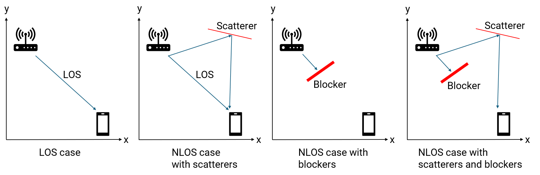
1. Non-Line-of-Sight (NLOS) Challenge: Indoor environments are cluttered with obstacles such as walls and furniture, which block direct line-of-sight (LOS) paths between anchors and the device. Additionally, indoor scatterers give rise to multipath propagation, where signals reflect and diffract, arriving at the receiver via multiple indirect paths. These multipath components often have longer travel distances and varying angles of arrival, significantly complicating the process of accurate localization.

2. Resolution Challenge: Indoor localization systems, such as those based on Wi-Fi, often operate with limited signal bandwidth and a small number of antennas. This restricts both range and angular resolution, making it difficult to distinguish between closely spaced positions and further degrading localization accuracy.

To address the NLOS challenge, fingerprinting-based methods have gained popularity. Unlike traditional techniques that use low-dimensional range and angle features, fingerprinting can leverage high-dimensional signatures—such as channel state information (CSI) or range-angle heatmaps which encapsulate rich environmental information, including NLOS effects. Deep learning models excel at extracting meaningful patterns from these complex, high-dimensional inputs, enabling direct mapping from signal fingerprints to precise position estimates.

To mitigate the resolution challenge, deploying multiple spatially distributed anchors is effective. While each anchor individually offers limited resolution, jointly processing the observations from multiple anchors can significantly enhance overall localization accuracy. However, fusing multi-view, high-dimensional perception data is non-trivial. Deep learning provides a powerful framework for integrating and processing these diverse features, enabling robust end-to-end localization even in challenging indoor environments.

Workflow Overview

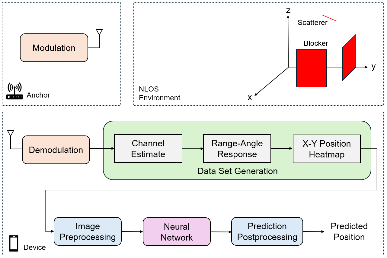
In this example, we consider an indoor environment equipped with multiple single-antenna wireless anchors and a multi-antenna target device. Each anchor periodically transmits OFDM-modulated signals in a coordinated manner (e.g., using a round-robin schedule) to avoid interference at the device. The device, knowing the positions of all anchors, receives signals from each anchor. Depending on the presence of obstacles (such as walls) and scatterers, the received signal at the device may be a direct line-of-sight (LOS) component, multipath components, or combination of both. For each anchor, the device demodulates the received OFDM signal to estimate the wireless channel.

From the estimated channel, the device computes a range-angle response, which characterizes the likely position of the device relative to each anchor. Using the known anchor positions, these responses are transformed into global X-Y coordinate heatmaps, representing the fingerprinting signatures of the device’s presence at each location in the room from the perspective of each anchor.

To leverage the spatial diversity provided by multiple anchors, the device aggregates the X-Y heatmaps from all anchors, stacking them into a multi-channel image. This image is preprocessed and then fed into a deep neural network—typically a convolutional neural network (CNN)—which is trained to infer the device’s position based on the combined information from all anchors. Finally, the neural network’s prediction is postprocessed to yield the estimated device position.

Scenario Configuration

For this example, we consider an indoor environment designed to challenge localization algorithms. The room is a rectangular space with dimensions 10 meters in length, 10 meters in width, and a height of 2 meters. The device to be localized is assumed to be held by a person at a height of approximately 1.5 meters above the floor.

% Scenario boundary in meters
boundLimit = [-5 5; ...                     % x_min x_max
    -5 5; ...                               % y_min y_max
    1.5 2];                                   % z_min z_max

The environment contains several key elements:

• Anchors: Six fixed anchors are deployed within the room. Each anchor is equipped with a single transmit antenna and operates at a carrier frequency of 5 GHz with a 20 MHz bandwidth.

• Scatterers and Blockers: To simulate multipath and NLOS conditions, the room includes three scatterers and four rectangular blockers (representing walls or large obstacles). The positions of anchors, scatterers, and blockers can be customized using the helperScenario function.

% Configure scenario
rng("default")
numAnchors = 6;
numScatterers = 3;
[scattererPos,anchorPos,anchorVel,rectBlockers] = helperScenario(boundLimit,numAnchors,numScatterers);

With a 20 MHz bandwidth, the theoretical one-way range resolution is given by $$\Delta R=c/B$$, where $$c$$ is the speed of light and $$B$$ is the bandwidth. This results in a range resolution of approximately 15 meters, which is relatively coarse compared to the room’s dimensions and limits localization accuracy.

% Configure RF parameters
fc = 5e9;                                        % Carrier frequency (Hz)
bw = 20e6;                                       % Bandwidth (Hz)
fs = bw;                                         % Sample rate (Hz)
c = physconst('LightSpeed');                     % Emission speed (m/s)
lambda = c/fc;                                   % Wavelength (m)

Each anchor uses a single isotropic transmit antenna. The device employs a uniform linear array (ULA) with $$M=8$$ critically spaced receive antenna elements $$\Delta \theta =\lambda /(Md)$$, where $$\lambda$$ is the wavelength at 5 GHz and $$d$$ is the antenna spacing. This configuration provides a boresight angle resolution of about 14 degrees, with poorer resolution at other angles, further constraining localization accuracy.

% Configure antennas
srcElement = phased.IsotropicAntennaElement(BackBaffled=false);
rxElement = phased.IsotropicAntennaElement(BackBaffled=false);
rxArray = phased.ULA(Element = rxElement, NumElements = 8, ElementSpacing=lambda/2);
txOrientationAxes = eye(3);
rxOrientationAxes = eye(3);

The system uses OFDM modulation, a standard in modern wireless communication. The OFDM waveform is configured for the 20 MHz channel with 64 subbands (data carriers). The frequency spacing is set accordingly, and the cyclic prefix (CP) length is chosen to exceed the maximum expected delay spread in the environment, ensuring robust channel estimation in the presence of multipath.

% Configure OFDM waveform
N = 64;                                          % Number of subbands (OFDM data carriers)
freqSpacing = bw/N;                              % Frequency spacing (Hz)
tsym = 1/freqSpacing;                            % OFDM symbol duration  (s)
rmax = 30;                                       % Maximum range of interest (m)
tcp = range2time(rmax);                          % Duration of the CP (s)
Ncp = ceil(fs*tcp);                              % Length of the CP in subcarriers
tcp = Ncp/fs;                                    % Adjusted duration of the CP (s)
tWave = tsym + tcp;                              % OFDM symbol duration with CP (s)
Ns = N + Ncp;                                    % Number of subcarriers in one OFDM symbol

The phased.ScatteringMIMOChannel object is used to model NLOS channels that account for multiple scatterers and the effects of LOS blockages. This setup enables the simulation of realistic NLOS conditions, capturing both direct and reflected signal paths.

% Configure transmitter and receiver
transmitter = phased.Transmitter('PeakPower',10);
receiver = phased.Receiver('NoiseFigure',10,'SampleRate',fs);

% Configure multipath channel
channel = cell(1,numAnchors);
for l = 1:numAnchors
    channel{l} = phased.ScatteringMIMOChannel('TransmitArray',srcElement, ...
        'ReceiveArray',rxArray,'PropagationSpeed',c,'CarrierFrequency',fc, ...
        'SampleRate',fs,'TransmitArrayMotionSource','Input port', ...
        'ReceiveArrayMotionSource','Input port','ScattererSpecificationSource','Property', ...
        'ScattererPosition',scattererPos,'ScattererCoefficient',ones(1,numScatterers), ...
        'SimulateDirectPath',true);
end

Data Set Generation

The data set generation process is designed to capture realistic measurements for training and evaluating the localization system. The procedure is as follows:

1. Data Collection: A person holding the device moves to various random positions within the room. At each position, the device simultaneously collects raw wireless signals transmitted from all anchors.

2. Channel Estimation: For each anchor, the device demodulates the received OFDM signal and estimates the wireless channel. This estimation accounts for both line-of-sight (LOS) and multipath components, depending on the presence of blockers and scatterers in the environment.

3. Range-Angle Response Calculation: Using the estimated channel data, the device computes the range-angle response for each anchor. This response characterizes the likely distance and direction of arrival of the signal components relative to the anchor.

4. Global X-Y Position Heatmap Generation: Since the positions of all anchors are known, the device transforms each anchor’s range-angle response into a spatial heatmap in the global X-Y coordinate domain. This transformation integrates the anchor’s location information, ensuring that all position images from different anchors correspond to the same region of interest (ROI) within the room.

The data set generation process is managed using the regenDataset flag. When regenDataset is set to true, the system generates the position heatmap data set, corresponding position labels, and the X and Y grid coordinates from scratch. This is accomplished by collecting raw data at random positions, demodulating the received signals, estimating the channels, and then computing the range-angle response using the phased.RangeAngleResponse object. The resulting responses are transformed into global X-Y position heatmaps via the helperPositionHeatmap utility, ensuring that all anchor data is referenced to a common ROI. Once the data set is generated, it is saved to a MAT file for future use.

If regenDataset is set to false, the data generation step is skipped, and the previously generated data set is loaded directly from the MAT file.

% Configure range-angle response
response = phased.RangeAngleResponse(SensorArray= rxArray, ...
    Mode = 'Bistatic', ...
    RangeMethod= 'FFT', ...
    ReferenceRangeCentered = true, ...
    OperatingFrequency= fc, SampleRate = fs,...
    SweepSlope = bw/tsym, ...
    RangeFFTLengthSource= 'Property', RangeFFTLength= 512, ...
    NumAngleSamples= 256, AngleSpan=[-180 180]);

% Configure position image helper
posHeatmap = helperXYPositionHeatmap(ROI = boundLimit(1:2,:));

% Dimensions of position image dataset
numSamples = 1000; 
imageSize = [81, 81, 1];

% Generate position image data set
regenDataset = false;
if regenDataset
    % Initialize position image dataset 
    dataset_images = zeros(imageSize(1), imageSize(2), imageSize(3), ... 
        numAnchors, numSamples); %#ok<UNRCH>
    dataset_labels = zeros(3,numSamples);

    % Generate position image dataset
    for sampleIdx = 1:numSamples
        % Generate random device positions
        [tgtPos,targetVel] = helperTargetPosition(boundLimit);

        % Truth label
        dataset_labels(:,sampleIdx) = tgtPos;

        % X-Y image generation: loop for different anchors
        for l = 1:numAnchors
            % BPSK symbol on each data carrier
            bpskSymbol = randi([0,1],[N 1])*2-1;

            % OFDM symbols
            sigmod = ifft(ifftshift(bpskSymbol,1),[],1);

            % OFDM symbols with cyclic prefix
            sig = sigmod([end-Ncp+(1:Ncp),1:end],:);

            % Power-normalized OFDM signal
            sig = sig/max(abs(sig),[],'all');

            % Transmitted signal
            signal = transmitter(sig);

            % Line-of-sight condition for each transmitter-receiver pair
            channel{l}.release();
            channel{l}.SimulateDirectPath = helperIsLineOfSight(tgtPos, anchorPos(:,l), rectBlockers);

            % Propagate signal for each transmitter-receiver pair
            sigp = channel{l}(signal,tgtPos,targetVel,txOrientationAxes, ...
                anchorPos(:,l),anchorVel(:,l),rxOrientationAxes);

            % Add receiver noise to collected signal
            sigr = receiver(sigp);

            % Remove the cyclic prefix
            sigrmvcp = sigr((Ncp+1):(Ncp+N),:);

            % Demodulate the received OFDM signal
            sigdemod = fftshift(fft(sigrmvcp,[],1),1);

            % Estimate channel
            chanest = conj(sigdemod./bpskSymbol);

            % Get range-angle response
            [raResp,rangeGrid,angleGrid] = response(chanest);

            % Generate X-Y position heatmaps
            rxPos = anchorPos(:,l);
            [x, y, xyr_mag_matrix] = posHeatmap.positionHeatMapData(raResp,rangeGrid,angleGrid,rxPos);
            dataset_images(:,:,:,l,sampleIdx) = xyr_mag_matrix; % (height, width, channels, anchors, samples)
        end
    end

    % Save the generated data set
    save('generated_data_set.mat', 'dataset_images', 'dataset_labels', 'x', 'y');
    fprintf('Data set saved as generated_data_set.mat\n');
else
    % Load the existing data set
    % load('generated_data_set.mat', 'dataset_images', 'dataset_labels', 'x', 'y');
    datasetZipFile = matlab.internal.examples.downloadSupportFile('phased','data/NLOSIndoorLocalizationData.zip');
    datasetFolder = fullfile(fileparts(datasetZipFile),'NLOSIndoorLocalizationData');
    if ~exist(datasetFolder,'dir')     
        unzip(datasetZipFile,datasetFolder);
    end
    file = load(fullfile(datasetFolder,"generated_data_set.mat"));
    dataset_images = file.dataset_images;
    dataset_labels = file.dataset_labels;
    x = file.x;
    y = file.y;
end

Single Instance Analysis

To gain deeper insight into the localization process, we examine a single representative case from the generated dataset. In this analysis, a specific target position is selected, and we explore the corresponding environment, line-of-sight (LOS) conditions, and position heatmaps.

caseIdx = 1;
tgtPosTest = dataset_labels(:,caseIdx);

First, we determine the LOS status between the target and each anchor. A status of 1 indicates a clear LOS path, while 0 indicates that the LOS path is obstructed by a wall or blocker.

% Line-of-sight conditions
los = true(1,numAnchors);
for l = 1:numAnchors
    los(l) = helperIsLineOfSight(tgtPosTest, anchorPos(:,l), rectBlockers);
end
display(los);

los = 1×6 logical array

   0   1   1   1   1   1

The scenario is visualized as follows:

• Anchors: Shown as blue upward-pointing triangles.

• Target Position: Indicated by a yellow dot.

• Scatterers: Marked with cyan stars.

• Blockers/Walls: Displayed as solid shapes within the room.

• LOS/NLOS Paths: Green lines connect anchors to the target where a clear LOS exists; red lines indicate blocked paths.

% Plot scenario
helperPlotScenario(rectBlockers,anchorPos,tgtPosTest,scattererPos,los);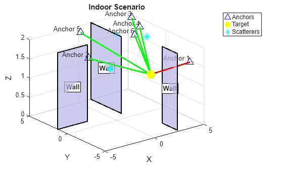

Next, we visualize the position heatmaps formed at the receiver using signals from each anchor. These heatmaps represent the likelihood of the target’s presence at different X-Y coordinates within the room. When a clear LOS path exists, the heatmap typically exhibits a pronounced peak at the target’s true location. However, in NLOS scenarios—where the LOS path is blocked or significant multipath from scatterers is present—the heatmap may become more diffuse or exhibit peaks at incorrect locations, reflecting the increased ambiguity in localization.

% Visualize position heatmap
f = figure;
los_status = strings(size(los));
los_status(los) = "LOS";
los_status(~los) = "NLOS";
for l = 1:numAnchors
    subplot(2,3,l,'Parent',f);
    XYImgTest = dataset_images(:,:,:,l,caseIdx); % (height, width, channels, anchors, samples)
    posHeatmap.plot(x, y, XYImgTest);
    title(sprintf('Anchor %d: %s',l,los_status(l)));
end

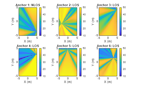
By analyzing these heatmaps and scenario visualizations, we gain a comprehensive understanding of how LOS and NLOS conditions impact the accuracy and reliability of position estimation in challenging indoor environments.

Data Preprocessing

To effectively utilize information from multiple anchors, we adopt an early fusion strategy. Specifically, we stack the position heatmaps from all anchors to form a multi-channel input image, where each channel corresponds to the heatmap from a different anchor.

% Reshape images: (height, width, channels, samples)
X = reshape(dataset_images, [imageSize(1), imageSize(2), imageSize(3)*numAnchors, numSamples]); 

Next, obtain training, validation, and testing index of data to support model development and unbiased performance evaluation.

% Ratios of training, validation and testing data
trainRatio = 0.8;
valRatio = 0.1;
testRatio = 0.1;

% Numbers of training, validation and testing data
numTrain = round(trainRatio * numSamples);
numVal = round(valRatio * numSamples);
numTest = numSamples - numTrain - numVal;

% Random partition
idx = randperm(numSamples);
trainIdx = idx(1:numTrain);
valIdx = idx(numTrain+1:numTrain+numVal);
testIdx = idx(numTrain+numVal+1:end);

Next, we perform input normalization to enhance the conditioning of the data for deep learning. To preserve the relative signal strength relationships across anchors, normalization parameters are computed globally from all heatmaps. We scale the pixel values such that the 1st percentile maps to 0 and the 99th percentile maps to 1, and then clamp all values to the ([0, 1]) range. To avoid the information from validation and testing data to influence normalization, we only use training data to calculate the percentiles.

% Training data
X_train = X(:,:,:,trainIdx);

% Percentiles from the training data
p1_global = prctile(X_train(:), 1);
p99_global = prctile(X_train(:), 99);

% Normalization of all input data using the percentiles
X_normalized = (X - p1_global) / (p99_global - p1_global);
X_normalized = max(0, min(1, X_normalized)); % clamp to [0,1]

The ground-truth X-Y position labels are also normalized to the ([0, 1]) interval based on the minimum and maximum values observed in the dataset. This normalization facilitates stable and efficient training of deep learning models.

% Spatial metadata
spatial_metadata.x_min = min(x);
spatial_metadata.x_max = max(x);
spatial_metadata.y_min = min(y);
spatial_metadata.y_max = max(y);

% Normalize labels to [0,1] range using spatial metadata
Y = dataset_labels(1:2,:); % (2, numSamples), output x-y coordinate only
Y_normalized = zeros(2, numSamples); 
Y_normalized(1,:) = (Y(1,:) - spatial_metadata.x_min) / ...
    (spatial_metadata.x_max - spatial_metadata.x_min); % x coordinates
Y_normalized(2,:) = (Y(2,:) - spatial_metadata.y_min) / ...
    (spatial_metadata.y_max - spatial_metadata.y_min); % y coordinates

Finally, convert the normalized data into dlarray format.

% Normalized training data
X_train = dlarray(X_normalized(:,:,:,trainIdx), 'SSCB'); % Spatial, Spatial, Channel, Batch
Y_train = dlarray(Y_normalized(:,trainIdx), 'CB');   % Channel, Batch

% Normalized validation data
X_val = dlarray(X_normalized(:,:,:,valIdx), 'SSCB');
Y_val = dlarray(Y_normalized(:,valIdx), 'CB');

% Normalized testing data
X_test = dlarray(X_normalized(:,:,:,testIdx), 'SSCB');
Y_test = dlarray(Y_normalized(:,testIdx), 'CB');
Y_test_original = Y(:,testIdx); % Keep original scale for evaluation

Network Architecture

We employ a convolutional neural network (CNN) to process the fused multi-channel heatmap images and predict the X-Y position of the target. The network architecture is designed as follows:

• Input Layer: The image input layer matches the dimensions of the early-fused images, where each channel corresponds to the heatmap from a different anchor.

• Feature Extraction: The network includes two 2D convolutional layers, each followed by a ReLU activation and a max pooling layer. The first convolutional layer uses 32 filters with a $$5\times 5$$ kernel, while the second layer uses 64 filters with a $$3\times 3$$kernel. These layers progressively extract low-level and high-level spatial features from the input images.

• Fully Connected Layers: After feature extraction, the output is flattened and passed through two fully connected layers. These layers learn to map the extracted features to the final X-Y position prediction.

• Output: The network outputs the predicted normalized X and Y coordinates of the target.

cnn_layers = [
    imageInputLayer([imageSize(1), imageSize(2), imageSize(3)*numAnchors])
    convolution2dLayer(5, 32, 'Padding', 'same')
    reluLayer
    maxPooling2dLayer(2, 'Stride', 2)
    convolution2dLayer(3, 64, 'Padding', 'same')
    reluLayer
    maxPooling2dLayer(2, 'Stride', 2)
    fullyConnectedLayer(128)
    reluLayer
    fullyConnectedLayer(2)  % Output: [x, y] position
    ];

Training Options

For network training, we utilize the Adam optimizer, which is well-suited for regression tasks. The training is performed with a mini-batch size of 32, and the data is shuffled at the beginning of every epoch to ensure robust learning and reduce the risk of overfitting.

The initial learning rate is set to $$1\times 10^{-4}$$. To facilitate steady convergence, we employ a piecewise learning rate schedule: the learning rate is reduced by a factor of 0.7 every 20 epochs. Training proceeds for a maximum of 30 epochs.

To further guard against overfitting, we incorporate early stopping based on validation performance. The model is evaluated on the validation set every 5 iterations. If the validation loss does not improve for 15 consecutive validation checks, training is halted early. This approach ensures that the model maintains good generalization without excessive training.

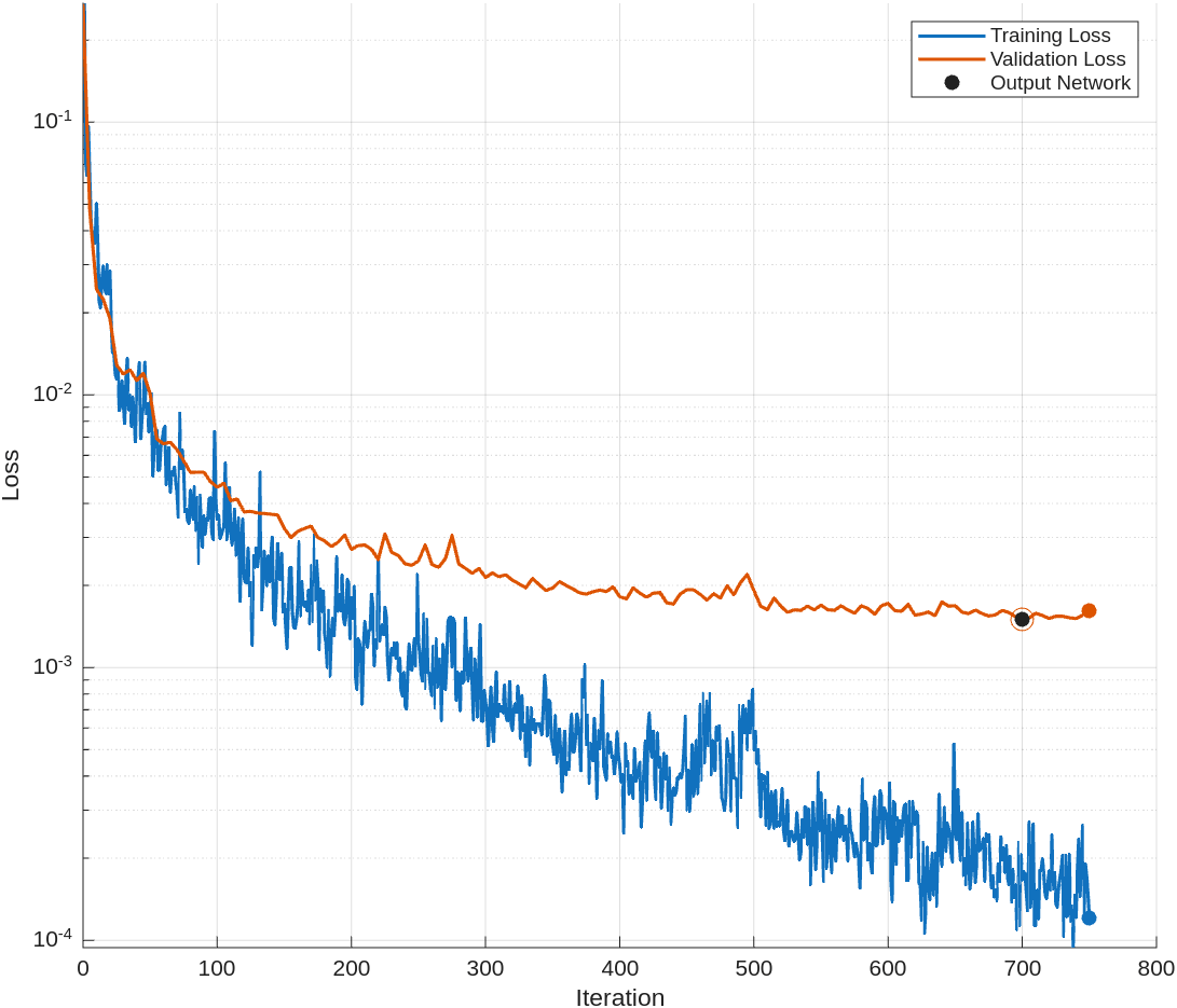
Throughout training, progress is monitored and visualized using training progress plots, and the training process is configured to run automatically on available computational resources.

options = trainingOptions('adam', ...
      MaxEpochs = 30, ...
      MiniBatchSize = 32, ...
      InitialLearnRate = 1e-4, ...
      Shuffle="every-epoch", ...
      LearnRateSchedule = 'piecewise', ...
      LearnRateDropFactor = 0.7, ...
      LearnRateDropPeriod = 20, ...
      ValidationData = {X_val, Y_val}, ...
      ValidationFrequency = 5, ...
      ValidationPatience = 15, ...
      Plots = 'training-progress', ...
      Verbose = true, ...
      ExecutionEnvironment = "auto");

Network Training

Since position estimation is a regression problem, we employ the mean squared error (MSE) as the loss function during training. This choice ensures that the network is optimized to minimize the average squared difference between the predicted and true X-Y coordinates.

The training process is controlled by the retrainNet flag. If retrainNet is set to true, the network is trained from scratch using the specified architecture, training options, and dataset. Upon completion, the trained model and associated metadata are saved for future use. If retrainNet is set to false, the training step is skipped and a pre-trained network is loaded from a MAT file.

It is important to note that the resulting trained model is tailored for the specific indoor environment in which the data was collected. If the deployment scenario or environment changes, the network should be retrained with new data to maintain accurate position estimation performance.

retrainNet = false;
if retrainNet
    net = trainnet(X_train, Y_train, cnn_layers, "mse", options); %#ok<UNRCH>
else
    % Load the existing network
    datasetZipFile = matlab.internal.examples.downloadSupportFile('phased','data/NLOSIndoorLocalizationModel.zip');
    datasetFolder = fullfile(fileparts(datasetZipFile),'NLOSIndoorLocalizationModel');
    if ~exist(datasetFolder,'dir')     
        unzip(datasetZipFile,datasetFolder);
    end
    file = load(fullfile(datasetFolder,"trained_network.mat"));
    net = file.net;
end

Evaluation and Visualization

To assess the performance of the trained model, we evaluate it on a separate test set. The model predicts the target positions, which are then denormalized to recover their original X-Y coordinates within the room.

% Make predictions on test data
Y_pred = predict(net, X_test);

% Denormalize predictions back to original coordinate scale
Y_pred_original = zeros(size(Y_pred));
Y_pred_original(1,:) = Y_pred(1,:) * (spatial_metadata.x_max - spatial_metadata.x_min) + ...
    spatial_metadata.x_min; % x coordinates
Y_pred_original(2,:) = Y_pred(2,:) * (spatial_metadata.y_max - spatial_metadata.y_min) + ...
    spatial_metadata.y_min; % y coordinates

Localization accuracy is quantified using the root mean squared error (RMSE) between the predicted and true positions. To provide a comprehensive understanding of the model's performance, we plot the cumulative distribution function (CDF) of the localization RMSE errors and report the total average localization RMSE error across all test samples.

% Calculate localization RMSE error for each test data point
loc_error = rmse(Y_test_original, Y_pred_original);

% Display localization RMSE error CDF
helperPlotLocErrorCDF(loc_error);

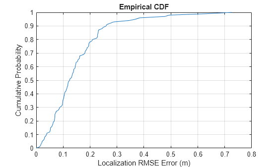
% Display total average localization RMSE error
loc_error_all = rmse(Y_test_original, Y_pred_original,'all');
fprintf('Total average localization RMSE error: %.3f meters\n', loc_error_all);

Total average localization RMSE error: 0.193 meters

In our experiments, the localization achieves sub-meter accuracy. This is a highly desirable outcome given the challenging NLOS indoor environment, where the underlying range resolution is about 15 meters and the boresight angle resolution is 14 degrees. These results demonstrate that the proposed deep learning approach significantly outperforms the limitations imposed by the physical signal resolutions.

The model's robustness to multipath and blockage is primarily attributed to the spatial diversity provided by multiple anchors. This setup with widely separated antennas also creates a large virtual aperture, enhancing the effective resolution. By processing multi-view information from different anchors, the deep learning model learns to exploit the underlying room geometry and infer the target's position with high accuracy, even under severe NLOS conditions.

Conclusion

This example demonstrates a comprehensive workflow for simulating and solving challenging indoor NLOS localization problems using fingerprinting and deep learning. By following this example, you can:

• Simulate Realistic NLOS Indoor Environments: The example demonstrates how to use phased.ScatteringMIMOChannel to create multipath channels with multiple scatterers and LOS blockage, capturing the complexity of real-world indoor environments.

• Generate Range-Angle Measurements and Position Heatmaps: With tools like phased.RangeAngleResponse and the custom helperPositionHeatmap objects, you can efficiently generate and preprocess X-Y position heatmaps from simulated measurements, forming a rich dataset suitable for deep learning applications.

• Build Deep Learning Models for Localization: The example shows how to structure and normalize data, and how to connect generated datasets to MATLAB’s deep learning functionality, such as designing and training CNNs for accurate position prediction.

• Evaluate and Visualize Performance: You can visualize NLOS indoor scenarios, evaluate localization accuracy using standard metrics (e.g., RMSE), display error distributions.

The workflow used in this example is adaptable and can be scaled to larger environments, different antenna configurations, and more complex channel conditions.

Reference

[1] Roshan Ayyalasomayajula, Aditya Arun, Chenfeng Wu, Sanatan Sharma, Abhishek Rajkumar Sethi, Deepak Vasisht, and Dinesh Bharadia. "Deep Learning based Wireless Localization for Indoor Navigation." In Proceedings of the 26th Annual International Conference on Mobile Computing and Networking, pp. 1-14. 2020.

[2] C. Wu et al., "Learning to Localize: A 3D CNN Approach to User Positioning in Massive MIMO-OFDM Systems," in IEEE Transactions on Wireless Communications, vol. 20, no. 7, pp. 4556-4570, July 2021.

[3] L. Italiano, B. Camajori Tedeschini, M. Brambilla, H. Huang, M. Nicoli and H. Wymeersch, "A Tutorial on 5G Positioning," in IEEE Communications Surveys & Tutorials, vol. 27, no. 3, pp. 1488-1535, June 2025.