Reduced-Order Modeling Technique for System-Level Simulation of Aircraft Wing Spar

This example shows how to run system-level simulations by using the Descriptor State-Space block to implement a reduced-order model of the I-beam in an aircraft wing spar. To complete the example, follow these steps:

1. Create a 3-D geometry of an I-beam and a finite-element model using Partial Differential Equation Toolbox™.

2. Reduce the finite-element model to have fewer degrees of freedom (DoFs) by using the Craig-Bampton reduced-order modeling (ROM) method.

3. Create reduced mass and stiffness matrices for use in the Descriptor State-Space block of the Simulink® model.

4. Model the coupling of aerodynamic loading and wing spar deflection in Simulink.

5. Simulate the beam deflection and loading by running a parameter sweep across different angles of attack and free-stream velocities.

6. Solve the full finite-element model for maximum deflection load by using the loading from the worst-case system-level simulation.

Open the model aeroelastic_feedback.slx containing the Descriptor State-Space block, Wing spar.

mdl = "aeroelastic_feedback";
open_system(mdl)

Create 3-D Geometry of I-Beam and Finite-Element Model

Create a geometry representing the cross-section of an I-beam, composed of rectangles for the web and flanges, both centered on the y-axis.

Define the geometric parameters of the I-beam.

tw = 0.015; % Thickness of the web
hw = 0.09; % Height of the web
tf = 0.02; % Thickness of the flange
wf = 0.08; % Width of the flange
spanOfBeam = 1.5;

Define the web cross-section using four rectangles that partition the web along the symmetric axes. Subdividing the web cross-section provides geometric vertices at the mid-web section, allowing application of lumped lift, drag, and twisting moment loads.

tw_sub = tw/2; % Subdivided web thickness - width for each rectangle
hw_sub = hw/2; % Subdivided web height - height for each rectangle

R1 = [3;4;-tw_sub;0;0;-tw_sub;-hw_sub;-hw_sub;0;0]; % Bottom left
R2 = [3;4;0;tw_sub;tw_sub;0;-hw_sub;-hw_sub;0;0]; % Bottom right
R3 = [3;4;-tw_sub;0;0;-tw_sub;0;0;hw_sub;hw_sub]; % Top left
R4 = [3;4;0;tw_sub;tw_sub;0;0;0;hw_sub;hw_sub]; % Top right

Define the rectangles for the flanges centered on the y-axis.

R5 = [3;4;-wf/2;wf/2;wf/2;-wf/2;
     hw_sub;hw_sub;hw_sub+tf;hw_sub+tf]; % Top flange
R6 = [3;4;-wf/2;wf/2;wf/2;-wf/2;
      -hw_sub;-hw_sub;-hw_sub-tf;-hw_sub-tf]; % Bottom flange

Create and plot a 2-D geometry of the cross-section.

geom_matrix = [R1, R2, R3, R4, R5, R6];
g = decsg(geom_matrix);
gm2D = fegeometry(g);

pdegplot(gm2D,FaceLabels="on")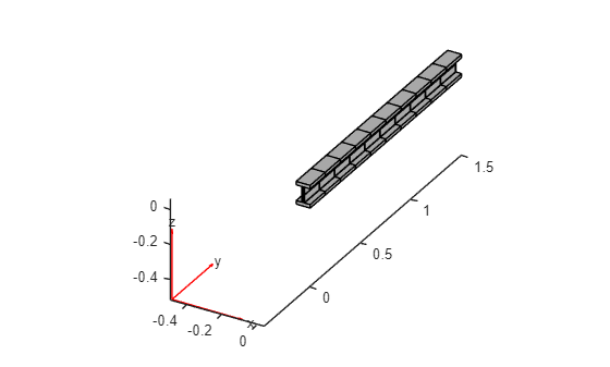

Create the 3-D beam geometry by extruding the 2-D cross-section along the total length of the wing spar. Create 10 sections along the beam's span by using a vector to specify the height of the extrusion. The numSections variable controls the number of extrusions.

numSections = 10;
extrusions = (spanOfBeam/numSections)*ones(numSections,1);
gm = extrude(gm2D,extrusions);

The extrude function extrudes a 2-D geometry along the z-axis. To match the typical orientation used in wing analysis, rotate the beam so that its span aligns with the y-axis and its deflection aligns with the z-axis.

gm = rotate(gm,-90,[0,0,0],[1,0,0]);

Plot the 3-D geometry.

figure
pdegplot(gm)

Create an femodel object for transient structural analysis, and include the I-beam geometry in the model.

model = femodel(AnalysisType="structuralTransient", ...
                Geometry=gm);

Specify Young's modulus, Poisson's ratio, and the mass density of the material.

model.MaterialProperties = ...
    materialProperties(YoungsModulus=210E9, ...
                       PoissonsRatio=0.3, ...
                       MassDensity=7800);

Generate the mesh.

model = generateMesh(model,Hmax=1);

Reduce Finite-Element Model to Fewer Degrees of Freedom

The Craig-Brampton reduced-order modeling (ROM) method computes the modal decomposition of a system and retains some of the physical degrees of freedom (DoFs) in the finite-element model. For this example, specify several interface locations where the DoFs are available in the reduced model as physical DoFs for applying loads and boundary conditions. The Craig-Bampton reduction process condenses the remaining DoFs into a few fixed-interface modes. Retain one vertex per section at the center of the I-beam to apply lift and drag loads. Additionally, keep a pair of vertices at each section to facilitate the application of twisting moments to the beam. Avoid the fixed end (y = 0) vertices by imposing the condition y > 0.

Locate the vertices at the center of the sections by using the coordinates x = 0 and z = 0.

centerVertexIDs = find(abs(gm.Vertices(:,1))<eps & ...
                       abs(gm.Vertices(:,3))<eps & ...
                       abs(gm.Vertices(:,2))>0);

Locate the vertices at the fore and aft of the web midline by using x =tw_sub and x =-tw_sub, respectively, and z = 0.

webForeVertexIDs = find(abs(gm.Vertices(:,1)-tw_sub)<eps & ...
                       abs(gm.Vertices(:,3))<eps & ...
                       abs(gm.Vertices(:,2))>0);
webAftVertexIDs = find(abs(gm.Vertices(:,1)+tw_sub)<eps & ...
                       abs(gm.Vertices(:,3))<eps & ...
                       abs(gm.Vertices(:,2))>0);

Locate the vertices on the fixed end.

fixedBCVertexIDs = find(abs(gm.Vertices(:,2))<eps);

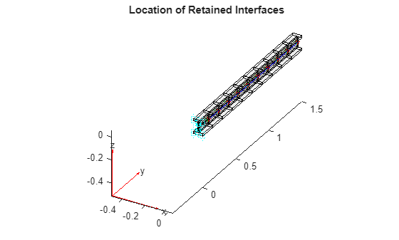
Plot the locations of the retained vertices. The red center vertices show the locations where drag and lift forces are applied. Simulate the twisting moment by applying equal and opposite forces at the green aft and blue fore locations.

figure
pdegplot(gm,FaceAlpha=0.1)
hold on
markVertices = @(gm,vertexIDs,markerSpec) ...
    plot3(gm.Vertices(vertexIDs,1),...
          gm.Vertices(vertexIDs,2),...
          gm.Vertices(vertexIDs,3),markerSpec);
markVertices(gm,webForeVertexIDs,"b");
markVertices(gm,webAftVertexIDs,"g*");
markVertices(gm,centerVertexIDs,"r*");
markVertices(gm,fixedBCVertexIDs,"cd");
title("Location of Retained Interfaces")

Define the ROM interfaces using all the loaded and fixed vertices.

romIntMid = romInterface(Vertex=...
                        [centerVertexIDs; ...
                         webForeVertexIDs; ...
                         webAftVertexIDs; ...
                         fixedBCVertexIDs]);

Assign the interface object to the ROMInterfaces property of the model.

model.ROMInterfaces = romIntMid;

Reduce the model while retaining all fixed-interface modes up to 10,000.

ROM = reduce(model,FrequencyRange=[-inf,10000]);

Create Reduced Mass and Stiffness Matrices

To simulate transient dynamics in Simulink:

• Apply proper constraints to the reduced mass and stiffness matrices available in the ROM to prevent rigid body motion.

• Identify the locations of various DoFs in the constrained ROM to apply loads and extract displacement from the solution.

First, create a function to retrieve the finite-element DoFs based on the geometric vertex IDs.

getFEDoFForVertex = ...
    @(msh,vertexIDs) findNodes(msh,"region",Vertex=vertexIDs)' ...
    + [0,1,2]*size(msh.Nodes,2);

The getFEDoFForVertex function returns a matrix with three columns, each corresponding to a spatial direction (x,y,z). Use this function to obtain the finite-element DoFs for all vertices of interest.

centerDoFs = getFEDoFForVertex(ROM.Mesh,centerVertexIDs);
webForeDoFs = getFEDoFForVertex(ROM.Mesh,webForeVertexIDs);
webAftDoFs = getFEDoFForVertex(ROM.Mesh,webAftVertexIDs);
fixedDoFs = getFEDoFForVertex(ROM.Mesh,fixedBCVertexIDs);

Apply the fixed boundary condition by eliminating the fixed DoFs from the ROM to obtain a properly constrained ROM system.

unconstrainedDOF = find(~ismember(ROM.RetainedDoF,fixedDoFs(:)));
modalDoF = numel(ROM.RetainedDoF) + (1:ROM.NumModes);
sysDof = [unconstrainedDOF;modalDoF'];
Kconstrained = ROM.K(sysDof,sysDof);
Mconstrained = ROM.M(sysDof,sysDof);

Next, create a dictionary to map all finite-element DoFs to their locations in the constrained ROM matrices, which already excludes the fixedDoFs. This dictionary assists in locating the DoFs corresponding to centerDoFs, webFwdDoFs, and webAftDoFs in the constrained ROM for load application.

ROMDoFs = setdiff(ROM.RetainedDoF,fixedDoFs(:));
MapROMDoF2Index = dictionary(ROMDoFs',1:numel(ROMDoFs));

Identify the locations of the DoFs corresponding to drag, lift, and twisting loads in the ROM.

centerDoFROMIdx = MapROMDoF2Index(centerDoFs);
webForeDoFROMIdx = MapROMDoF2Index(webForeDoFs);
webAftDoFROMIdx = MapROMDoF2Index(webAftDoFs);
DragDoFROMIdx = centerDoFROMIdx(:,1);
LiftDoFROMIdx = centerDoFROMIdx(:,3);
foreXROMIdx = webForeDoFROMIdx(:,1);
foreZROMIdx = webForeDoFROMIdx(:,3);
aftXROMIdx = webAftDoFROMIdx(:,1);
aftZROMIdx = webAftDoFROMIdx(:,3);

Apply damping, and expand the second-order time system to a first-order system. Create the reduced mass and stiffness matrices, Mode and Kode, to use in the Simulink model.

alpha = 0.001;
beta = 0.1;
nDoF = size(Mconstrained,1);
Mode = [speye(nDoF,nDoF),sparse(nDoF,nDoF); ...
        alpha*Mconstrained+beta*Kconstrained,Mconstrained];
Kode = [sparse(nDoF,nDoF),-speye(nDoF,nDoF); ...
        Kconstrained,sparse(nDoF,nDoF)];

Model Aerodynamic Loads and Wing Spar Deflection

The Simulink aeroelastic_feedback.slx model uses the aerodynamic lift, drag, and moment coefficients to provide force inputs to the finite-element model at discrete locations, or stations, along the span-wise locations. The aerodynamic forces and moments are coupled with the structural dynamics, because the deformation of the wing causes a change in the air flowing around the wing. Feed the deformation of the finite-element model back into the aerodynamic calculations to capture this aeroelastic phenomenon.

The forces generated in the area between these stations are concentrated at a point load at the quarter chord location, according to the conventions of aerodynamic coefficients. Simulink calculates the aerodynamic forces and moments using these equations:

$\text{Lift}=\frac{1}{2}\rho V_{\infty }^{2}S{C}_L$, $\text{Drag}=\frac{1}{2}\rho V_{\infty }^{2}S{C}_D$, $\text{Moment}=\frac{1}{2}\rho V_{\infty }^{2}Sc{C}_M$.

Here, $\rho$ is the air density, $V_{\infty }$is the airspeed, S is the wing area, C is the aerodynamic coefficient, and c is the chord length. Define the parameters for the Simulink model.

nStations = length(find(aftZROMIdx));
AEROELASTIC = 1; % Turn load-deformation coupling on/off in model
chord = 1.0;
areas = chord*extrusions;
rho = 1.225;

The Simulink model uses the aerodynamic coefficients in a lookup table with the angle of attack as the query variable. Apply the loads, and then read the deformation in 10 span locations. The axis conventions cause air to flow over the wing in the positive x-direction, and a positive moment corresponds to a node-up pitching moment.

data = readmatrix("airfoil_coeffs.csv");
coeffs = data(:,[1:3 5]); % Save only lift, drag, moment

Each span-wise location has four inputs and four outputs. Define them in the order in which they are used in Simulink. Create the moment at each station by applying two forces on the beam model, but in opposite directions. Apply the forces at the same distance from the axis of rotation (the y-axis): one force at a negativex-location and another at a positive x-location. The forces have equal magnitudes in the z-direction: one in the positive z-direction and another in the negative z-direction.

Input

• Lift force (z-direction)

• Drag force (x-direction)

• Forward component of moment (positive x-location)

• Aft component of moment (negative x-location)

inIdx = [LiftDoFROMIdx,DragDoFROMIdx, ...
         foreZROMIdx,aftZROMIdx]';
inIdx = inIdx(:);

Output

• Forward x-deflection

• Aft x-deflection

• Forward z-deflection

• Aft z-deflection

outIdx = [foreXROMIdx,aftXROMIdx, ...
          foreZROMIdx,aftZROMIdx]';
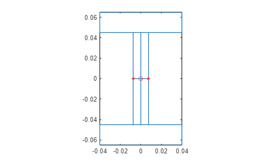
outIdx = outIdx(:);

Plot the cross-section of the l-beam, and use a red circle to indicate the lift and drag forces acting on the center location of the cross-section. Indicate the mesh nodes corresponding to the moment forces and the deflection outputs using red asterisks on the edge of the web of the cross-section.

figure
pdegplot(gm2D)
hold on
plot(0,0,"ro")
plot([-tw_sub,tw_sub],[0,0],"r*")
hold off

Organize the input and output vectors to stack the four data points at each span location on top of each other. The B matrix of the DSS system ensures that you apply the input forces at the correct state indexes.

nIn = length(inIdx);
Bbot = sparse(nDoF,nIn);
Bbot(inIdx' + (0:nDoF:((nIn-1)*nDoF))) = 1;
Brom = [sparse(nDoF,nIn); Bbot];

Create the C matrix so that the system returns only the necessary deflection information.

nOut = length(outIdx);
Ctop = sparse(nDoF,nOut);
Ctop(outIdx' + (0:nDoF:((nOut-1)*nDoF))) = 1;
Crom = [Ctop; sparse(nDoF,nOut)]';

Create a function to save the test parameters and maximum deflection to the SimulationOutput object.

function out = postsim(out,aoa,q)
    out.deflection = out.yout(end);
    out.AOA = aoa;
    out.q = q;
end

Simulate Beam Deflection

With the system defined, run the model across a sweep of operating conditions that vary the angle of attack and free-stream air velocity.

mdl = "aeroelastic_feedback";
sweepAOA = -16.75:19.25;
sweepVinf = 100:50:250;

clear in
in(1:numel(sweepAOA)*numel(sweepVinf)) = Simulink.SimulationInput(mdl);
in = reshape(in,numel(sweepAOA),numel(sweepVinf));

for i = 1:numel(sweepAOA)
    for j = 1:numel(sweepVinf)
        aoai = sweepAOA(i);
        qi = 0.5*rho*sweepVinf(j)*sweepVinf(j);
        in(i,j) = setBlockParameter(in(i,j), ...
         'aeroelastic_feedback/AOA wrt Root',...
         'Bias',num2str(aoai));
        in(i,j) = setBlockParameter(in(i,j), ...
         'aeroelastic_feedback/Apply aerodynamic loads and moments/Dynamic Presssure (q)', ...
         'Gain',num2str(qi));
        in(i,j) = setPostSimFcn(in(i,j), @(x) postsim(x,aoai,qi));
    end
end

out = parsim(in,TransferBaseWorkspaceVariables="on", ...
                ShowProgress="off");

Starting parallel pool (parpool) using the 'Processes' profile ...
20-Jan-2026 16:42:19: Job Queued. Waiting for parallel pool job with ID 1 to start ...
20-Jan-2026 16:43:19: Job Queued. Waiting for parallel pool job with ID 1 to start ...
Connected to parallel pool with 6 workers.

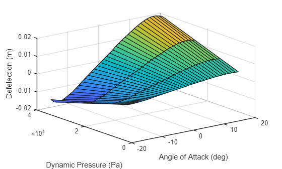
Plot the maximum deflection of each test point by using the SimulationOutput object.

X = zeros(size(out));
Y = zeros(size(out));
Z = zeros(size(out));

for i = 1:size(out,1)
    for j = 1:size(out,2)
        X(i,j) = out(i,j).AOA;
        Y(i,j) = out(i,j).q;
        Z(i,j) = out(i,j).deflection;
    end
end


surf(X,Y,Z);
xlabel("Angle of Attack (deg)");
ylabel("Dynamic Pressure (Pa)");
zlabel("Deflection (m)")

openSimulationManager(in,out)

After a sweep, you can use the resulting highest stress operating conditions as input to the high-fidelity finite-element solver and run the analysis to determine the efficacy of the wing spar.

Solve Full Finite-Element Model for Maximum Deflection Load

Find the index of maximum deflection loading and apply those loads. Because aeroelastic coupling affects the load, you must fetch the coupled load from the Simulink output and apply it to all stations of the model.

[v,idx] = max(Z,[],"all");

maxAOA = X(idx);
maxDynamicPresssure = Y(idx);

stations = numel(extrusions);
AeroDynamicLoad = out(idx).logsout{1}.Values.Data(end,:);
AeroDynamicLoad = reshape(AeroDynamicLoad,[],stations);

The AeroDynamicLoad matrix includes lift in the first row, drag in the second row, and the couple forming the twisting moment in the last two rows. The number of columns corresponds to the number of stations.

LiftForce = AeroDynamicLoad(1,:);
DragForce = AeroDynamicLoad(2,:);
MomentCoupleFwd = AeroDynamicLoad(3,:);
MomentCoupleAft = AeroDynamicLoad(4,:);

In Partial Differential Equation Toolbox, apply the force as a three-element vector at each vertex. First, construct a 3-by-n matrix to apply at three sets of vertices: the center of the station, and the forward and aft vertices at the mid-web section. Here, n is the number of stations.

centerVerticesForce(1,:) = DragForce;
centerVerticesForce(3,:) = LiftForce;
webFwdVerticesForce(3,:) = MomentCoupleFwd;
webAftVerticesForce(3,:) = MomentCoupleAft;

Unassigned rows default to zero values in these assignments. Loop through the columns to apply the force vector at three sets of vertices at each station.

for i = 1:stations
    model.VertexLoad(centerVertexIDs(i)) = ...
        vertexLoad(Force=centerVerticesForce(:,i));
    model.VertexLoad(webForeVertexIDs(i)) = ...
        vertexLoad(Force=webFwdVerticesForce(:,i));
    model.VertexLoad(webAftVertexIDs(i)) = ...
        vertexLoad(Force=webAftVerticesForce(:,i));
end

Before simulating the full model, apply the fixed constraint and specify the damping parameters.

model.VertexBC(fixedBCVertexIDs) = vertexBC(Constraint="fixed");
model.DampingAlpha = alpha;
model.DampingBeta = beta;

Solve the model.

tlist = 0:0.01:1;
Rtransient = solve(model,tlist);

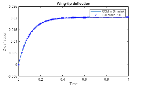
Compare the bending deflection at the wing tip obtained with the full model to the deflection obtained with ROM simulated in Simulink.

figure
plot(out(idx).tout,out(idx).yout)
hold on
nodeAtWingTipWebAft = ...
     getFEDoFForVertex(model.Mesh,webAftVertexIDs(end));
plot(Rtransient.SolutionTimes, ...
Rtransient.Displacement.uz(nodeAtWingTipWebAft(:,1),:),'b*')
title("Wing-Tip Deflection")
xlabel("Time")
ylabel("Z-Deflection")
legend("ROM in Simulink","Full-Order PDE")

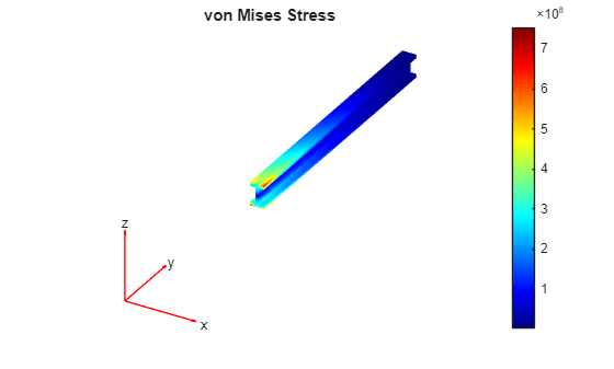
The full model solution also contains stresses in the model. Plot the von Mises stress.

figure
VMstress = Rtransient.evaluateVonMisesStress;
pdeplot3D(model.Mesh,ColorMapData=VMstress(:,end))
title("von Mises Stress")