Using Scale Factors to Facilitate MPC Weights Tuning

This example shows how to specify scale factors in an MPC controller to make weights tuning easier.

Define Plant Model

The discrete-time, linear, state-space plant model has 10 states, 5 inputs, and 3 outputs.

[plant,Ts] = mpcscalefactor_model;
[ny,nu] = size(plant.D);

The plant inputs include manipulated variable (MV), measured disturbance (MD) and unmeasured disturbance (UD). The plant outputs include measured outputs (MO) and unmeasured outputs (UO).

MVindex = [1, 3, 5];
MDindex = 4;
UDindex = 2;
MOindex = [1 3];
UOindex = 2;
plant = setmpcsignals(plant, ...
    'MV',MVindex, ...
    'MD',MDindex, ...
    'UD',UDindex, ...
    'MO',MOindex, ...
    'UO',UOindex);

The nominal values and operating ranges of plant model are as follows:

• Input 1: manipulated variable, nominal value is 100, range is [50 150]

• Input 2: unmeasured disturbance, nominal value is 10, range is [5 15]

• Input 3: manipulated variable, nominal value is 0.01, range is [0.005 0.015]

• Input 4: measured disturbance, nominal value is 0.1, range is [0.05 0.15]

• Input 5: manipulated variable, nominal value is 1, range is [0.5 1.5]

• Output 1: measured output, nominal value is 0.01, range is [0.005 0.015]

• Output 2: unmeasured output, nominal value is 1, range is [0.5 1.5]

• Output 3: measured output, nominal value is 100, range is [50 150]

Define and Analyze Open-Loop Plant Signals

Use lsim command to run an open loop linear simulation to verify that plant outputs are within the range and their average are close to the nominal values when input signals vary randomly around their nominal values.

% set input and output range
Urange = [100;10;0.01;0.1;1];
Yrange = [0.01;1;100];

% set input and output nominal values
% for this example nominal values are equivalent to ranges
Unominal = [100;10;0.01;0.1;1];
Ynominal = [0.01;1;100];

% define time intervals
t = (0:1000)'*Ts;
nt = length(t);

% define input and output signals
Uol = (rand(nt,nu)-0.5).*(ones(nt,1)*Urange');   % design input signal
Yol = lsim(plant,Uol,t);                        % compute plant output

fprintf(['The differences between average output values ' ...
    '\n and the nominal values are: ' ... 
    ' %.2f%%, %.2f%%, %.2f%% respectively.\n'], ...
    abs(mean(Yol(:,1)))/Ynominal(1)*100, ...
    abs(mean(Yol(:,2)))/Ynominal(2)*100, ...
    abs(mean(Yol(:,3)))/Ynominal(3)*100);

The differences between average output values 
 and the nominal values are:  1.29%, 2.05%, 2.29% respectively.

Display means and standard deviations of input and output signals.

% input
mean(Uol)

ans = 1×5

    0.6246   -0.1146   -0.0000    0.0010    0.0010

std(Uol)

ans = 1×5

   28.3381    2.9129    0.0029    0.0282    0.2805

% output
mean(Yol)

ans = 1×3

    0.0001    0.0205   -2.2864

std(Yol)

ans = 1×3

    0.0032    0.3691   31.1872

Here, the mean values give a good idea of the actual nominal values and the standard deviation capture some idea of the range.

Evaluate MPC with Default MPC Weights

When plant input and output signals have different orders of magnitude, default MPC weight settings often give poor performance.

Create an MPC controller with default weights:

• Weight.MV = 0

• Weight.MVRate = 0.1

• Weight.OV = 1

% create mpc object
mpcobjUnscaled = mpc(plant);

-->"PredictionHorizon" is empty. Assuming default 10.
-->"ControlHorizon" is empty. Assuming default 2.
-->"Weights.ManipulatedVariables" is empty. Assuming default 0.00000.
-->"Weights.ManipulatedVariablesRate" is empty. Assuming default 0.10000.
-->"Weights.OutputVariables" is empty. Assuming default 1.00000.

% nominal values of the plant states
Xnominal = zeros(10,1);

% nominal values for unmeasured disturbance (must be 0)
Unominal(UDindex) = 0;

% Set nominal values
mpcobjUnscaled.Model.Nominal = struct( ...
    'X',Xnominal, ...
    'DX',Xnominal, ...
    'Y',Ynominal, ...
    'U',Unominal);

To calculate plant outputs, sim will subtract the nominal plant inputs from the inputs, and the nominal states from the current states, then apply the linear plant equations, and finally add the nominal output values to the calculated output.

To calculate the manipulated variables, it will remove the nominal output from the plant output signal, calculate the MPC control sequence, and add the nominal value of the manipulated variables to the calculated sequence.

First, test a sequence of step setpoint changes in three reference signals.

% expected step response duration
nStepLen = 15;

% calculate simulation time to accommodate ny steps   
Ns1 = nStepLen*ny;

% reference signal
r1 = ones(Ns1,1)*Ynominal(:)';

% cycle through each output and define references at StepLen intervals
StepTime = 1;
for i = 1:ny
    r1(StepTime:end,i) = r1(StepTime:end,i) + Yrange(i);
    StepTime = StepTime + nStepLen;
end

% simulate closed loop for Ns1 steps and subject to reference r1
sim(mpcobjUnscaled,Ns1,r1)

-->The "Model.Disturbance" property is empty:
   Assuming unmeasured input disturbance #2 is integrated white noise.
-->Assuming output disturbance added to measured output #1 is integrated white noise.
   Assuming no disturbance added to measured output #3.
-->"Model.Noise" is empty. Assuming white noise on each measured output.

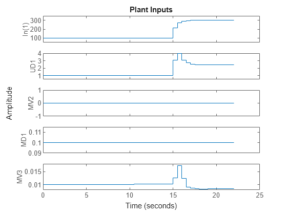
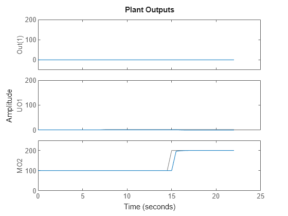
The tracking response of the first output is poor. The reason is that its range is small compared to the other outputs. If the default controller tuning weights are used, the MPC controller does not pay much attention to regulating this output because the associated penalty is so small compared to the other outputs in the objective function.

Second, test the unmeasured disturbance rejection.

% create simulation options object and set unmeasured disturbance
SimOpt = mpcsimopt;
SimOpt.UnmeasuredDisturbance = Urange(UDindex)';

% set number of simulation steps and reference signal 
% reference signal is equal to the range values
Ns2 = 100;
r2 = ones(Ns2,1)*Yrange(:)'; 

% simulate the closed loop subject to reference r2 
sim(mpcobjUnscaled,Ns2,r2,[],SimOpt)

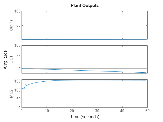
The disturbance rejection response is also poor. None of the outputs return to their setpoints.

Evaluate MPC with Default MPC Weights After Specifying Scale Factors

Specifying input and output scale factors for the MPC controller:

• Improves the numerical quality of the optimization and state estimation calculations.

• Makes it more likely that the default tuning weights will achieve good controller performance.

Copy the MPC controller with default weights.

mpcobjScaled = mpcobjUnscaled;

To specify scale factors, it is good practice to use the expected operating range of each input and output.

% scale manipulated variables
for i = 1:length(MVindex)
    mpcobjScaled.ManipulatedVariables(i).ScaleFactor = ...
        Urange(MVindex(i));
end

% scale measured disturbances
nmd = length(MDindex);
for i = 1:nmd
    mpcobjScaled.DisturbanceVariables(i).ScaleFactor = ...
        Urange(MDindex(i));
end

% scale unmeasured disturbances
for i = 1:length(UDindex)
    mpcobjScaled.DisturbanceVariables(i+nmd).ScaleFactor = ...
        Urange(UDindex(i));
end

% scale outputs
for i = 1:ny
    mpcobjScaled.OV(i).ScaleFactor = Yrange(i);
end

Repeat the first test, which is a sequence of step setpoint changes in three reference signals.

sim(mpcobjScaled,Ns1,r1)

-->The "Model.Disturbance" property is empty:
   Assuming unmeasured input disturbance #2 is integrated white noise.
-->Assuming output disturbance added to measured output #1 is integrated white noise.
   Assuming no disturbance added to measured output #3.
-->"Model.Noise" is empty. Assuming white noise on each measured output.

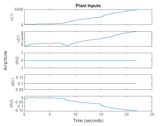
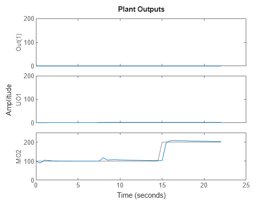
Repeat the second test, which is an unmeasured disturbance.

sim(mpcobjScaled,Ns2,r2,[],SimOpt)

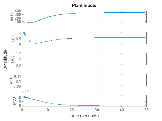
Both setpoint tracking and disturbance rejection responses are good even without tuning MPC weights. This is because now the original weights apply to scaled signals, and therefore the weighting effect is not distorted.