Mapped CI Lookup Tables as Functions of Fuel Mass and Engine Speed
The Model-Based Calibration Toolbox™ includes projects and templates that you can use to generate calibrated compression-ignition (CI) lookup tables as a function of fuel mass and engine speed. Use the tables in the Powertrain Blockset™ Mapped CI Engine (Powertrain Blockset) block.
Use Test Plan Template to Fit Models
In the Model Browser, to open the data, select Import Data. Navigate to the spreadsheet that contains the data.
For example, open
matlab\toolbox\mbc\mbctraining\CiEngineData.xlsx.The spreadsheet contains firing and motor data collected at different engine torques and speeds.
Firing Data Description FuelMassCmd Commanded fuel mass, in mg
Torque Engine torque, in Nm
EngSpd Engine speed, in rpm
AirMassFlwRate Air mass flow, in kg/s
BSFC Engine brake-specific fuel consumption (BSFC), in g/kWh
CO2MassFlwRate Carbon dioxide emission mass flow, in kg/s
COMassFlwRate Carbon monoxide emission mass flow, in kg/s
ExhTemp Exhaust temperature, in K
FuelMassFlwRate Fuel mass flow, in kg/s
HCMassFlwRate Hydrocarbon emission mass flow, in kg/s
NOxMassFlwRate Nitric oxide and nitrogen dioxide emissions mass flow, in kg/s
PMMassFlwRate Particulate matter emission mass flow, in kg/s
Nonfiring motor data is collected at different engine speeds, without fuel consumption.
Nonfiring Data Description Torque Engine torque command, in Nm
EngSpd Engine speed, in rpm
AirMassFlwRate Air mass flow, in kg/s
In the Select Sheet dialog box, select the data that you want to calibrate. For example, select
Firing Data.Optionally, use the Data Editor filter the data. After you have filtered the data, close the Data Editor.
In the Model Browser, select Fit Models. In the Fit Models dialog box, in the Template pane, select the template.
For example, to fit the firing data in the spreadsheet, select
MappedEngine-Fuel. Do not change the default responses and inputs.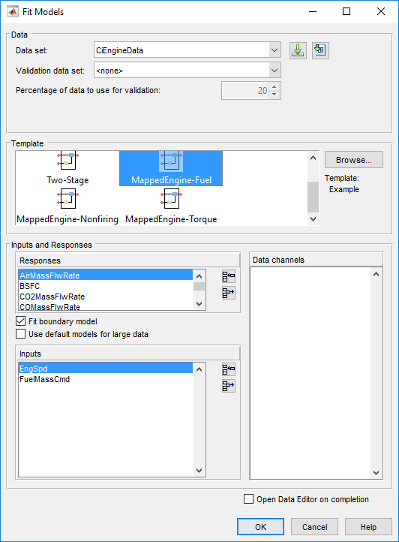
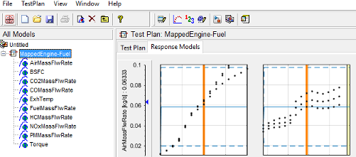
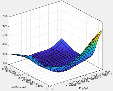
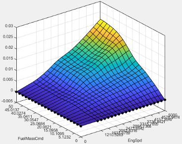
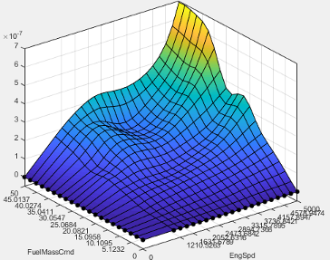
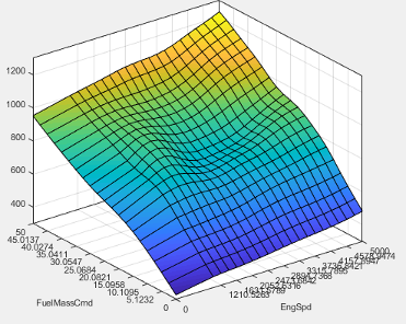
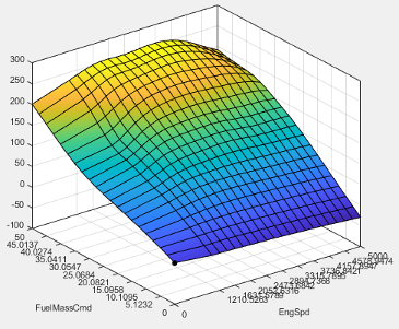
Review the model fits.
To review the response models, in the tree, select the top level.
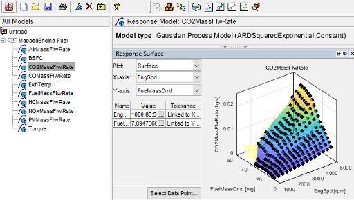
To review the response surfaces, in the tree, select the response.
Open CAGE Project
To open the project, in the CAGE Case Studies pane:
Select
CI Mapped Engine - Fuel Input.Click Open Example.
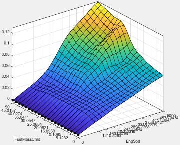
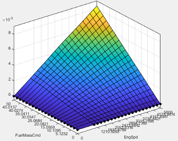
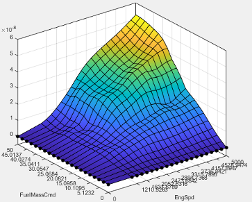
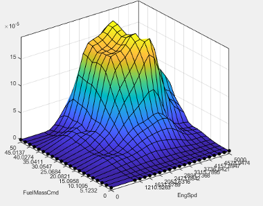
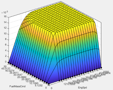
The project includes these tables.
| Name | Description | Table |
|---|---|---|
| Air mass flow, in kg/s |
|
| Engine brake-specific fuel consumption (BSFC), in g/kWh |
|
| Carbon dioxide emission mass flow, in kg/s |
|
| Carbon monoxide emission mass flow, in kg/s |
|
| Exhaust temperature, in K |
|
f_fuel | Fuel mass flow, in kg/s |
|
| Hydrocarbon emission mass flow, in kg/s |
|
| Nitric oxide and nitrogen dioxide emissions mass flow, in kg/s |
|
| Particulate matter emission mass flow, in kg/s |
|
| Engine torque command, in Nm |
|
Use CAGE to Import and Replace Models
Use the project to import and replace existing models with new models.
In CAGE, select File > Import > Model. If you do not have a model open, the model browser opens. Select a model.
If your current project has two or more test plans, the Import Models dialog box prompts you to merge compatible models. Select No.
The Import Models dialog box prompts you to
Replace,Skip, orCreate newmodels. SelectReplace.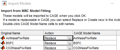
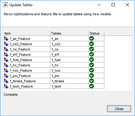
After you import and replace the existing models, the Import Models wizard opens the Update Tables dialog box. You can use the Update Table dialog box to rerun optimizations and feature fills to update the tables with the new models.
Review and Export Lookup Tables
In CAGE, review the calibrated tables.
To export the tables, select File > Export > Calibration > All Items. Use the Export to parameter to specify the format. To export so that you can use the data for the Powertrain Blockset mapped engine blocks, select
Simulink Model
                    Workspace
. The Model-Based Calibration Toolbox saves the mapped engine table and breakpoint data to the model workspace.
See Also
Mapped CI Engine (Powertrain Blockset)