Specify Presample and Forecast Period Data to Forecast ARIMAX Model

This example shows how to partition a timeline into presample, estimation, and forecast periods, and it shows how to supply the appropriate number of observations to initialize a dynamic model for estimation and forecasting.

Consider estimating and forecasting a dynamic model containing autoregressive and moving average terms, and a regression component for exogenous predictor variables (for example, an ARMAX model). To estimate and forecast the model, estimate must have enough presample responses to initialize the autoregressive terms, and it must have enough innovations to initialize the moving average terms. If you do not specify presample responses, then estimate backcasts for the required amount, and it sets the required presample innovations to 0.

Similarly, to forecast responses from the fitted model, forecast must have enough presample responses and innovations. Although you must specify presample responses, forecast sets required presample innovations to 0. Further, the regression component in the forecast period requires forecasted or future predictor data; without future predictor data, forecast drops the regression component from the model when it generates forecasts.

Although the default behaviors of estimate and forecast are reasonable for most workflows, a good practice is to initialize a model yourself by partitioning the timeline of your sample into presample, estimation, and forecast periods, and supplying the appropriate amount of observations.

Consider an ARMAX(1,2) model that predicts the current US real gross national product (GNPR) rate with the current industrial production index (IPI), employment (E), and real wages (WR) rates as exogenous variables. Partition the timeline of the sample into presample, estimation, and forecast periods. Fit the model to estimation sample, and use the presample responses to initialize the autoregressive term. Then, forecast the GNPR rate from the fitted model. When you forecast:

• Specify responses at the end of the estimation period as a presample to initialize the autoregressive term

• Specify predictor data at the end of the estimation period as a presample to initialize the moving average component. forecast infers the required innovations from the specified presample responses and predictor data.

• Include the effects of the predictor variables on the forecasted responses by specifying future predictor data.

Load the Nelson-Plosser data set.

load Data_NelsonPlosser

For details on the data set, display Description.

The table DataTable contains yearly measurements, but the data set is agnostic of the time base. To apply the time base to the data, convert DataTable to a timetable.

DataTable = table2timetable(DataTable,"RowTimes",datetime(DataTable.Dates,"Format","yyyy"));

Among the series in DataTable, some of the sample start dates begin in different years. DataTable synchronizes all series by prepending enough leading NaNs so that all series have the same number of elements.

Econometrics Toolbox™ ARIMA model software removes all rows (time points) from the response and predictor data if at least one observation is missing. This default behavior can complicate timeline partitioning. One way to avoid the default behavior is to remove all rows containing at least one missing value yourself.

Remove all leading NaNs from the data by applying listwise deletion.

varnames = ["GNPR" "IPI" "E" "WR"];
Tbl = rmmissing(DataTable(:,varnames));

Stabilize the response and predictor variables by converting them to returns.

StblTbl = varfun(@price2ret,Tbl);
StblTbl.Properties.VariableNames = varnames;
T = size(StblTbl,1) % Total sample size

T = 
61

GNPR = StblTbl.GNPR;
X = StblTbl{:,varnames(2:end)};

Conversion to returns reduces the sample size by one.

To fit an ARMAX(1,2) model to the data, estimate must initialize the conditional mean of the first response ${\mathit{y}}_1$ by using the previous response ${\mathit{y}}_0$ and the two previous innovations ${\epsilon }_0$ and ${\epsilon }_{-1}$. If you do not specify the presample values, estimate backcasts to obtain ${\mathit{y}}_0$ and it sets presample innovations to 0, which is their expected value.

Create index vectors for presample, estimation, and forecast samples. Consider a 5-year forecast horizon.

idxpresample = 1;
idxestimate = 2:56;
idxforecast = 57:T;

Fit an ARMAX(1,2) model to the data. Specify the presample response data and estimation-sample exogenous data. Because there is no model from which to derive presample innovations, allow estimate to set the required presample innovations to 0.

Mdl = arima(1,0,2);

y0est = GNPR(idxpresample); % Presample response data for estimation
yest = GNPR(idxestimate);   % Response data for estimation 
XEst = X(idxestimate,:);     % Estimation sample exogenous data

Mdl = estimate(Mdl,yest,'Y0',y0est,'X',XEst,'Display','off');

To forecast an ARMAX(1,2) model into the forecast period, forecast must initialize the first forecast ${\mathit{y}}_{57}$ by using the previous response ${\mathit{y}}_{56}$and the previous two innovations ${\epsilon }_{56}$ and ${\epsilon }_{55}$. However, if you supply enough response and exogenous data to initialize the model, then forecast infers innovations for you. To forecast an ARMAX(1,2) model, forecast requires the three responses and the two observations from the exogenous data just before the forecast period. When you provide presample data for forecasting, forecast uses only the latest required observations. However, this example proceeds by specifying only the necessary amount of presample observations.

Forecast the fitted ARMAX(1,2) model into the forecast period. Specify only the necessary observations at the end of the estimation sample as presample data. Specify the forecast period exogenous data.

y0f = yest((end - 2):end); % Presample response data for forecasting
X0f = XEst((end - 1):end,:); % Presample exogenous data for forecasting
XF = X(idxforecast,:);     % Forecast period exogenous data for model regression component

yf = forecast(Mdl,5,y0f,'X0',X0f,'XF',XF);

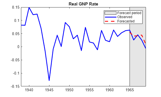
yf is a 5-by-1 vector of forecasted responses representing the continuation of the estimation sample yest into the forecast period.

Plot the latter half of the response data and the forecasts.

yrs = year(StblTbl.Time(30:end));

figure;
plot(yrs,StblTbl.GNPR(30:end),"b","LineWidth",2);
hold on
plot(yrs(end-4:end),yf,"r--","LineWidth",2);
h = gca;
px = yrs([end - 4 end end end - 4]);
py = h.YLim([1 1 2 2]);
hp = patch(px,py,[0.9 0.9 0.9]);
uistack(hp,"bottom");
axis tight
title("Real GNP Rate");
legend(["Forecast period" "Observed" "Forecasted"])