Deploy Direction of Arrival Estimation Using Deep Learning on Desktop
This example shows how to generate and deploy code to estimate direction of arrival (DOA) using deep learning techniques within an Intel® desktop environment using Simulink®. This example uses model reference blocks to conduct software-in-the-loop (SIL) simulations that collect the execution time metrics of the generated code.
Complete the Direction-of-Arrival Estimation Using Deep Learning example to understand the fundamentals of direction of arrival estimation with deep learning.
This example extends the data set preparation, training procedures, and post-processing steps from the Direction-of-Arrival Estimation Using Deep Learning example to develop a complete deployment workflow.
Data set to Train Deep Learning Network
Simulate a dataset using Phased Array System Toolbox™, following the setup in the Direction-of-Arrival Estimation Using Deep Learning example. Key configuration details include:
ULA configuration: 8 receivers
Multiple SNR scenarios for diverse noise powers
Each sample: 200 received signal snapshots
Covariance matrices (real and imaginary parts) as CNN input
Use the helperGenerateTrainData function to generate the data set by simulating the received signals at the ULA under the specified conditions.
dataset = helperGenerateTrainData();
Estimation DOA Using Deep Learning
Deep DOA Estimator Model
This example casts DOA estimation as a multi-label classification problem, so the deep learning model in this example:
Uses covariance matrices derived from array snapshots (real & imaginary channels) as inputs.
Outputs a probability vector over incident angles of length 181 (–90° to 90°, 1° resolution).
The example uses a convolutional neural network (CNN) to map the input covariance matrices to the probability vector over incident angles. In this implementation, the network uses fewer layers and fewer filters per layer than the architecture in the Direction‑of‑Arrival Estimation Using Deep Learning example, while maintaining comparable performance. This streamlined design better supports the deployment workflow shown in this example.
kern_size1 = 3;
kern_size2 = 2;
m = size(dataset.trainData,1);
angleGrid = -90:1:90;

r = length(angleGrid);
layers = [
    imageInputLayer([m m 2],Normalization="none")

    convolution2dLayer(kern_size1, 64, Padding="same")
    batchNormalizationLayer()
    reluLayer()

    convolution2dLayer(kern_size2, 64, Padding="same")
    batchNormalizationLayer()
    reluLayer()

    convolution2dLayer(kern_size2, 64, Padding="same")
    batchNormalizationLayer()
    reluLayer()

    fullyConnectedLayer(512)
    reluLayer()
    dropoutLayer(0.3)

    fullyConnectedLayer(256)
    reluLayer()
    dropoutLayer(0.3)

    fullyConnectedLayer(r,WeightsInitializer="glorot")
    sigmoidLayer()
    ];
The optimized architecture provides a 96% reduction in the trained model footprint, which is critical for real-time deployment.
Train the Network
Train the model using the weighted cross-entropy loss function for improved learning at true source locations.
function loss = customLoss(y,t) %#ok<DEFNU>
    loss = crossentropy(y,t,t*10+1,ClassificationMode="multilabel");
end

metric = accuracyMetric(ClassificationMode="multilabel");

options = trainingOptions("adam", ...
    InitialLearnRate=1e-4, ...
    MaxEpochs=2000, ...
    MiniBatchSize=5000, ...
    Shuffle="every-epoch", ...
    Verbose=true, ...
    Plots="training-progress", ...
    ExecutionEnvironment="auto", ...
    Metrics=metric, ...
    OutputNetwork="last-iteration");
You can skip this training by using a pretrained network. If you want to train the network as the example runs, set trainNow to true. If you want to skip the training steps and load a MAT file containing the pretrained network, set trainNow to false.
trainNow =false; if trainNow deepDOAEstimator = trainnet(dataset.trainData,dataset.trainLabels,... layers,@(y,t)customLoss(y,t),options); %#ok<UNRCH> else if (exist("deepDOAEstimator.mat",'file') ~= 2) zipFile = matlab.internal.examples.downloadSupportFile("dsp","DeepDOAEstimator.zip"); dataFolder = fileparts(zipFile); unzip(zipFile,cd) end file = load("deepDOAEstimator.mat"); deepDOAEstimator = file.deepDOAEstimator; end
Visual Comparison: Deep Learning vs. MUSIC
After training, randomly select an observation from the validation set and compare the Multiple Signal Classification (MUSIC) estimator's pseudospectrum with the deep DOA estimator's learned target probability over angles using the helper function helperPlotDOASpectrum. The dotted lines on the plots mark the true angle locations.
rng("default");
idxToCompare= randi(length(dataset.validIdx),[1,4]);
helperPlotDOASpectrum(deepDOAEstimator,dataset,idxToCompare)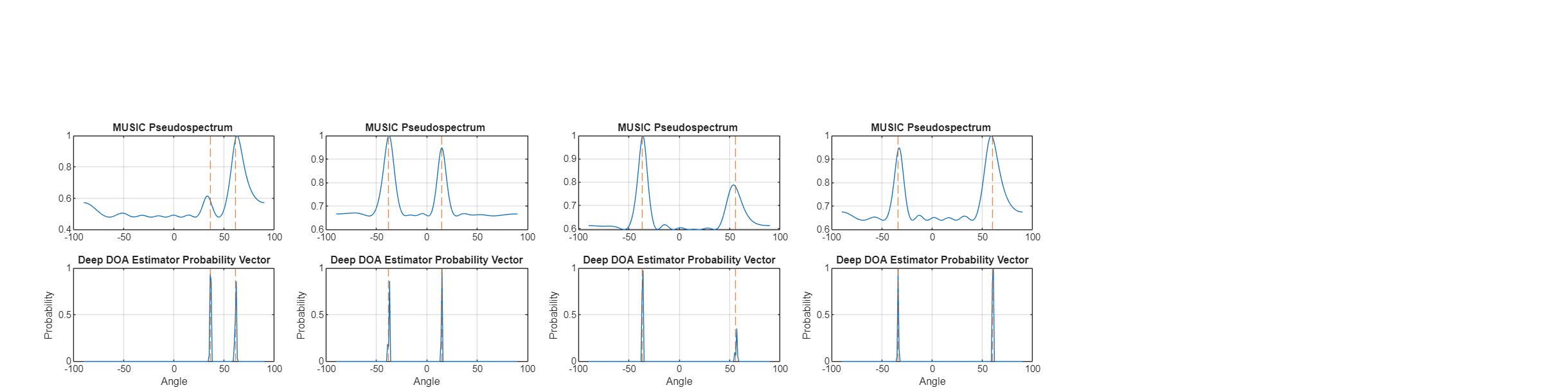
Both methods exhibit distinct peaks at the directions where sources exist. However, the peaks from the deep DOA estimator are sharper even with a significantly smaller network
Evaluate Performance of Deep DOA Estimator
You can compare the performance of the deep DOA estimator and the MUSIC estimator under various scenarios as outlined in the Direction-of-Arrival Estimation Using Deep Learning example. This example compares the performances across various SNR levels.
Performance Comparison Across SNR Scenarios
Compare the performance of the deep DOA estimator and the MUSIC estimator under different SNR scenarios by varying the SNR from -15 dB to 1 dB, using fixed angle pairs of 10 and 15 degrees, which are close to the center of angle grid.
The helper function helperCompareDOAOverSNR generates data at each SNR, predicts DOA using MUSIC and deep DOA estimator and plots the computed average estimation error.
dBSNRList = -15:2:1;
sourceAngles = [10,15];
helperCompareDOAOverSNR(deepDOAEstimator,dBSNRList,sourceAngles)
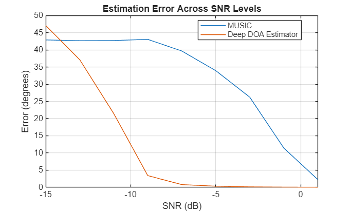
Both methods accurately estimate angles at high SNR levels, but the deep DOA estimator maintains relatively good accuracy even under low SNR conditions. Even under SNR conditions lower than those in the training data, the deep DOA estimator remains stable, demonstrating strong generalization ability across different SNR scenarios.
Simulink model
Open the Simulink model attached to this example. Use this model to simulate the DOA estimation workflow. This model implements DOA estimation using the trained deep learning model and MUSIC algorithm and compares the execution times using Software-in-the-Loop Simulation (Embedded Coder) simulation.
topMdl = 'DOAMainModel';
open_system(topMdl)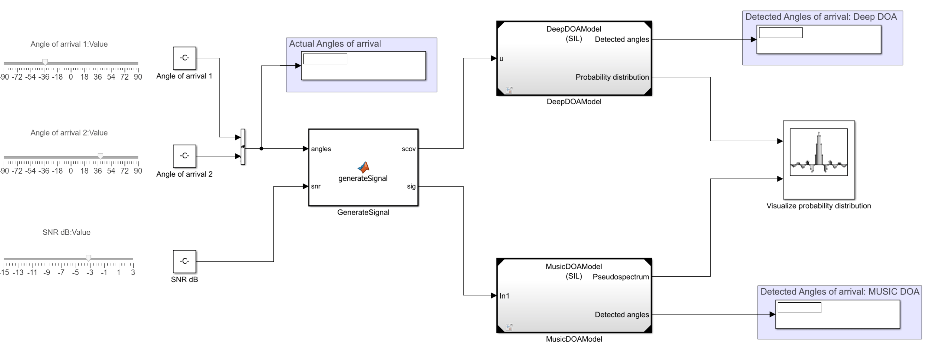
Adjust the sliders for angles of arrival and SNR values to set the desired parameters. You can modify these parameters at run time. The GenerateSignal subsystem utilizes a MATLAB Function (Simulink) block to simulate the received signal at the ULA using sources at the specified angles, leveraging the capabilities of Phased Array System Toolbox™.
function [scov,sig] = generateSignal(angles,snr)
    noisePwr = db2pow(-snr);
    NumElements = 8;
    fc = 300e6;
    Nsnapshots = 500;
    lambda = physconst("LightSpeed")/fc;
    ula = phased.ULA(NumElements=NumElements, ...
        ElementSpacing=lambda/2);
    pos = getElementPosition(ula) / lambda;

    [sig,~,scov] = sensorsig(pos, Nsnapshots, [angles; 0*angles], noisePwr);
end
The MusicDOAModel and DeepDOAModel models, which implement the MUSIC and deep learning algorithms respectively, use resulting signal and covariance matrix.
refMdlDOA = 'DeepDOAModel';
load_system(refMdlDOA);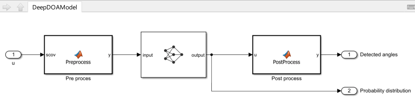
The deep learning-based DOA estimation algorithm uses a Predict (Deep Learning Toolbox) block, which runs the network trained as described in earlier steps. To ensure compatibility with CNNs, the covariance matrix is separated into real and imaginary components before being passed to the Predict block. The resulting probability vector is then processed to detect the angles of arrival. In this example, the number of sources is fixed and assumed to be known, with exactly two sources present. The probability distribution can be visualized using the Array Plot block. The display blocks also highlight the detected angles of arrival.
refMdlMUSIC = 'MusicDOAModel';
load_system(refMdlMUSIC);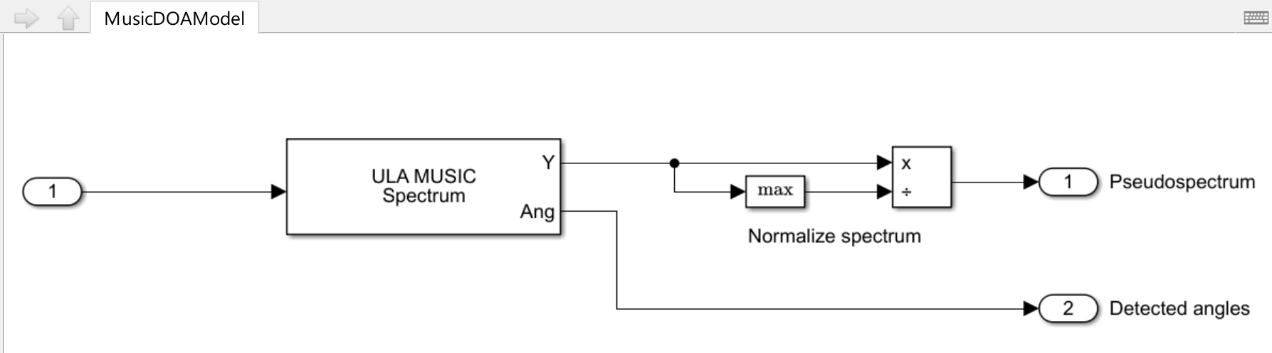
MUSIC DOA estimation is carried out using the ULA MUSIC Spectrum block, which generates the MUSIC spatial spectrum. This spectrum is then normalized to allow direct comparison with the probability distribution computed by the Predict block.
Desktop deployment
You can configure the referenced model interactively by using the Configuration Parameters dialog box from the Simulink model toolstrip, or programmatically by using the MATLAB command-line interface.
Configure Model Using UI
To configure a referenced Simulink model to generate code, complete these steps for both referenced models MusicDOAModel and DeepDOAModel.
Open the referenced Simulink model. In the Modeling tab of the referenced model, click Model Settings to open the Configuration Parameters dialog box.
In the Hardware Implementation pane, set the Device vendor parameter to
Intel. Set the Device type parameter tox86-64(Windows 64)orx86-64(Linux 64)based on your desktop environment.In the Code Generation pane:
Set System target file to
ert.tlc.Set Build configuration to
Faster Runsto prioritize execution speed.
Under Code Generation, in the Code Style pane, set Dynamic array container type to
coder::array.In the Simulation Target pane, enable Dynamic memory allocation in MATLAB functions.
Open the top model, right-click the corresponding reference model and set Simulation mode to
Software-in-the-loop (SIL).
Configure Model Using Programmatic Approach
Alternatively, you can set all the configurations using set_param commands.
Set the Device vendor parameter to Intel. Set the Device type parameter to x86-64 (Windows 64) or x86-64 (Linux 64) based on your desktop environment.
set_param(refMdlDOA,'HardwareBoard','None')
set_param(refMdlMUSIC,'HardwareBoard','None')
if strcmp(computer('arch'),'win64')
set_param(refMdlDOA,'ProdHWDeviceType','Intel->x86-64 (Windows64)')
    set_param(refMdlMUSIC,'ProdHWDeviceType','Intel->x86-64 (Windows64)')
elseif strcmp(computer('arch'),'glnxa64')
    set_param(refMdlDOA,'ProdHWDeviceType','Intel->x86-64 (Linux 64)')
    set_param(refMdlMUSIC,'ProdHWDeviceType','Intel->x86-64 (Linux 64)')
end
Select 'ert.tlc' as the system target file to optimize the code for embedded real-time systems, and choose 'Faster Runs' for the build configuration to prioritize execution speed.
set_param(refMdlDOA,'SystemTargetFile','ert.tlc')
set_param(refMdlDOA,'BuildConfiguration','Faster Runs')

set_param(refMdlMUSIC,'SystemTargetFile','ert.tlc')
set_param(refMdlMUSIC,'BuildConfiguration','Faster Runs')
Enable dynamic memory allocation for MATLAB functions. Set the dynamic array container type to 'coder::array'.
set_param(refMdlDOA,'MATLABDynamicMemAlloc','on')
set_param(refMdlDOA,'DynamicArrayContainerType','coder::array')

set_param(refMdlMUSIC,'MATLABDynamicMemAlloc','on')
set_param(refMdlMUSIC,'DynamicArrayContainerType','coder::array')
Enable code execution profiling to analyze the performance of the code.
set_param(refMdlDOA,'CodeExecutionProfiling','on')
set_param(refMdlMUSIC,'CodeExecutionProfiling','on')

close_system(refMdlDOA,1)
close_system(refMdlMUSIC,1)
Set the Simulation mode parameter of the model reference block to 'Software-in-the-loop (SIL)' to generate the code for the referenced model and use the code for SIL simulation.
set_param([topMdl '/' refMdlDOA],'SimulationMode','Software-in-the-loop (SIL)')
set_param([topMdl '/' refMdlMUSIC],'SimulationMode','Software-in-the-loop (SIL)')
Run the parent model to initiate code generation from the referenced Simulink model and use the model for SIL simulation.
Configure the parent model to check if the model works in real time. In the Apps tab of the Simulink model toolstrip, click the SIL/PIL Manager app. Set System Under Test to 'Model blocks in SIL/PIL Mode' and enable Task Profiling. Click on Run Verification to start profiling.
Increase the Stop Time to simulate the model for a longer duration.
sim(topMdl);
### Searching for referenced models in model 'DOAMainModel'.
### Total of 2 models to build.
### Starting serial code generation build.
### Starting build procedure for: DeepDOAModel
### Model reference code generation target for DeepDOAModel is up to date.
### Starting serial code generation build.
### Starting build procedure for: MusicDOAModel
### Successful completion of build procedure for: MusicDOAModel

Build Summary

Model reference code generation targets:

Model          Build Reason                             Status                        Build Duration
====================================================================================================
MusicDOAModel  Model or library MusicDOAModel changed.  Code generated and compiled.  0h 2m 7.2967s

1 of 2 models built (1 models already up to date)
Build duration: 0h 2m 21.163s
### Preparing to start SIL simulation ...
### Preparing to start SIL simulation ...
Building with 'MinGW64 Compiler (C)'.
MEX completed successfully.
### Starting SIL simulation for component: MusicDOAModel
### Starting SIL simulation for component: DeepDOAModel
### Application stopped
### Stopping SIL simulation for component: MusicDOAModel
### Application stopped
### Stopping SIL simulation for component: DeepDOAModel
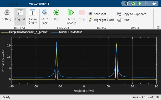
Tune the sliders for the angles of arrival and SNR controls while the model is running to observe the pseudospectrum. Even at low SNR levels, the deep DOA estimator produces a sharper distribution.
Profiling results
Execution‑time measurements were collected using software‑in‑the‑loop (SIL) simulation on an Intel® Xeon® W‑2133 CPU (6 physical cores, 12 logical processors, 3.6 GHz base frequency) and 64 GB RAM running Windows 11 OS.
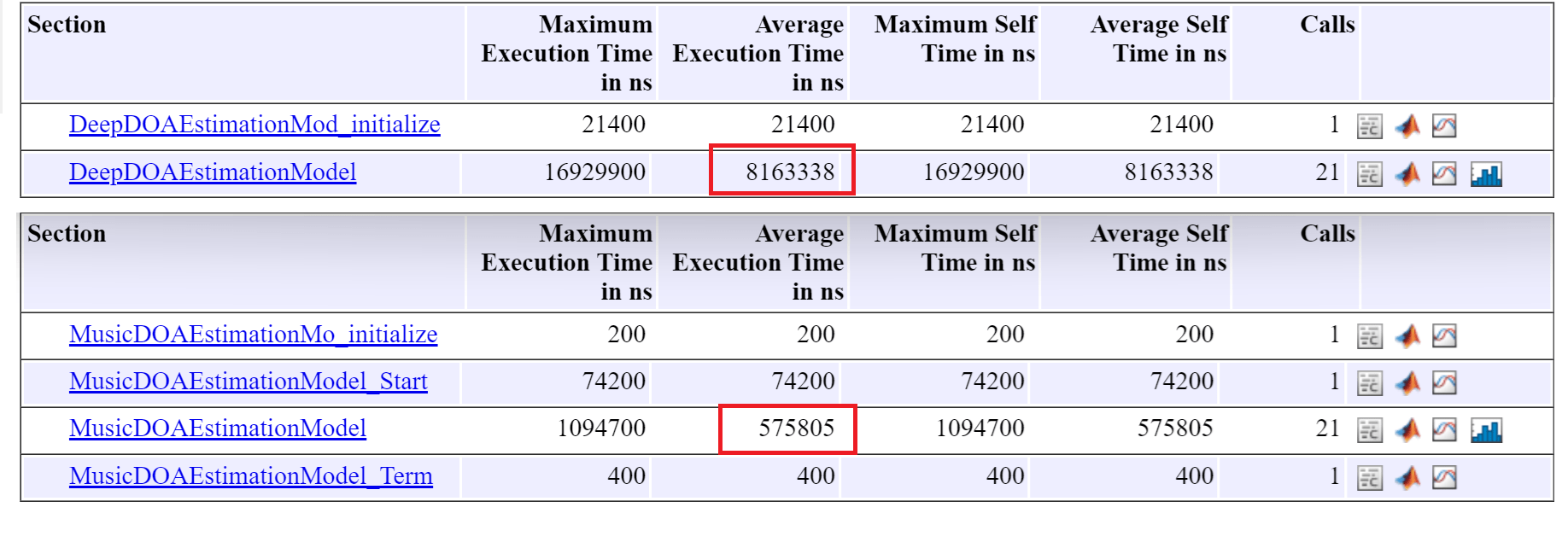
In this example, the average execution time for the step function in the deep DOA detector (8.2 ms) is considerably higher than that of the MUSIC DOA detector (0.56 ms), as expected. However, both runtimes are sufficiently low to support reliable real‑time deployment.