Arbitrary Magnitude Filter Design
This example shows how to design filters with arbitrary magnitude response. The family of filter design (FDESIGN) objects allow for the design of filters with various types of responses. Among these types, the arbitrary magnitude is the less specialized and most versatile one. The examples below illustrate how arbitrary magnitude designs can solve problems when other response types find limitations.
FIR Modeling with the Frequency Sampling Method
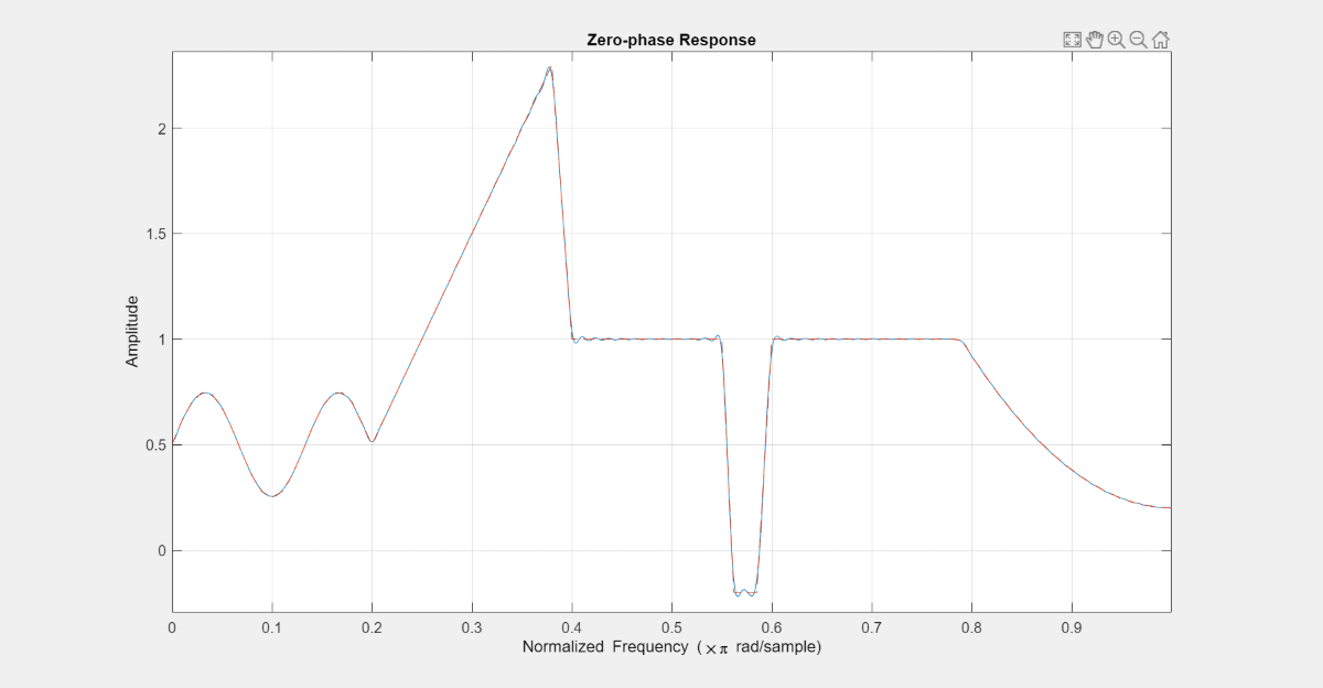
This section illustrates a case where the amplitude of the filter is defined over the complete Nyquist range (there are no relaxed or "don't care" regions). The example that follows uses a single (full) band specification type and the robust frequency sampling algorithm to design a filter whose amplitude is defined over three sections: a sinusoidal section, a piecewise linear section and a quadratic section. It is necessary to select a large filter order because the shape of the filter is quite complicated:
N = 300;
B1 = 0:0.01:0.18;
B2 = [.2 .38 .4 .55 .562 .585 .6 .78];
B3 = 0.79:0.01:1;
A1 = .5+sin(2*pi*7.5*B1)/4;    % Sinusoidal section
A2 = [.5 2.3 1 1 -.2 -.2 1 1]; % Piecewise linear section
A3 = .2+18*(1-B3).^2;          % Quadratic section
F = [B1 B2 B3];
A = [A1 A2 A3];
d = fdesign.arbmag('N,F,A',N,F,A);
Hd = design(d,'freqsamp','SystemObject',true);
fvtool(Hd,'MagnitudeDisplay','Zero-phase');
close(gcf)
In the previous example, the normalized frequency points were distributed between 0 and pi rad/sample (extrema included). You can also specify negative frequencies and obtain complex filters. The following example models a complex RF bandpass filter and uses a Kaiser window to mitigate the effects of the Gibbs phenomenon that occurs due to the 70 dB magnitude gap between the -pi and pi rad/sample frequencies:
load cfir.mat; % load a predefined set of frequency and amplitude vectors
N = 200;
d = fdesign.arbmag('N,F,A',N,F,A);
Hd = design(d,'freqsamp', 'window' ,{@kaiser,20},'SystemObject',true);
fvtool(Hd,'FrequencyRange','[-pi, pi)');

Modeling Smooth Functions with an Equiripple FIR Filter
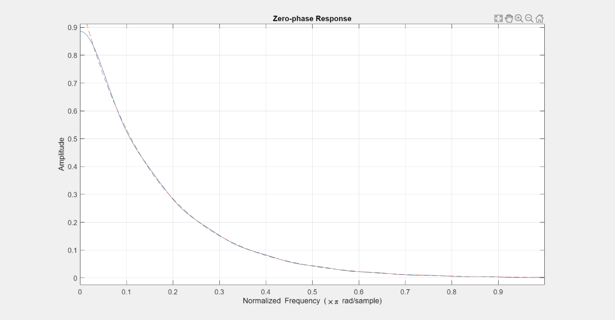
The equiripple algorithm is well suited for modeling smooth functions as shown in the following example that models an exponential with a minimum order FIR filter. The example specifies a small ripple value across all frequencies and defines weights that increase proportionally to the desired amplitude to improve the performance at high frequencies:
F = linspace(0,1,100);
A = exp(-2*pi*F);
R = 0.045; % ripple
W = .1-20*log10(abs(A)); % weights
d = fdesign.arbmag('F,A,R',F,A,R);
Hd = design(d,'equiripple','weights',W,'SystemObject',true);
fvtool(Hd,'MagnitudeDisplay','Zero-phase', 'FrequencyRange','[0, pi)');
Single-Band vs. Multi-Band Equiripple FIR Designs
In certain applications, it might be of interest to shape the stopband of the filter to, for example, minimize the integrated side-lobe levels, or to improve the quantization robustness. The following example designs a lowpass filter with a staircase stopband. To achieve the design, it uses a distribution of weights that increase the attenuation of each step by 5 dB in the stopband:
N = 150;
F = [0 .25 .3 .4 .401 .5 .501 .6 .601 .7 .701 .8 .801 .9 .901 1];
A = [1 1 0 0 0 0 0 0 0 0 0 0 0 0 0 0];
W = 10.^([0 0 5 5 10 10 15 15 20 20 25 25 30 30 35 35]/20);
d = fdesign.arbmag('N,F,A',N,F,A);
Hd1 = design(d,'equiripple','weights',W,'SystemObject',true);
The following example presents an alternative design based on the use of a multi-band approach that defines two bands (passband and stopband) separated by a "don't care" region (or transition band):
B = 2;            % Number of bands
F1 = F(1:2);      % Passband
F2 = F(3:end);    % Stopband
% F(2:3)=[.25 .3] % Transition band
A1 = A(1:2);
A2 = A(3:end);
W1 = W(1:2);
W2 = W(3:end);
d = fdesign.arbmag('N,B,F,A',N,B,F1,A1,F2,A2);
Hd2 = design(d,'equiripple','B1Weights',W1,'B2Weights',W2,...
    'SystemObject',true);
hfvt = fvtool(Hd1,Hd2,'MagnitudeDisplay','Magnitude (dB)','Legend','On');
legend(hfvt, 'Single-Band Design', 'Multi-Band Design');
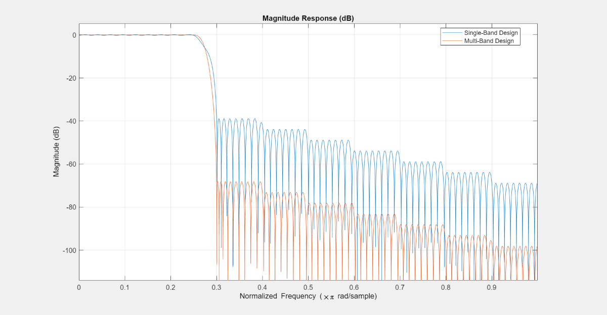
Notice the clear advantage of the multi-band approach. By relaxing constraints in the transition region, the equiripple algorithm converges to a solution with lower passband ripples and greater stopband attenuation. In other words, the frequency characteristics of the first filter could be matched with a lower order. The following example illustrates this last comment by obtaining equivalent filters using minimum order designs.
Minimum order designs require the specification of one ripple value per band. For this example, set the ripple to 0.0195 in all bands.
R = 0.0195;

% Single-band minimum order design
d = fdesign.arbmag('F,A,R',F,A,R);
Hd1 = design(d,'equiripple','Weights',W,'SystemObject',true);

% Multi-band minimum order design
d = fdesign.arbmag('B,F,A,R',B,F1,A1,R,F2,A2,R);
Hd2 = design(d,'equiripple','B1Weights',W1,'B2Weights',W2,...
    'SystemObject',true);

hfvt = fvtool(Hd1,Hd2);
legend(hfvt, 'Single-Band Minimum Order Design', ...
  'Multi-Band Minimum Order Design');

The passband ripple and stopband attenuation of both designs match. However, the single-band design has an order of 152 while the multi-band design has an order of 72.
order(Hd)
ans = 32
Constrained Multi-Band Equiripple Designs
Multi-band equiripple designs allow you to specify ripple constraints for different bands, specify single-frequency bands, and force specified frequency points to specified values.
Constrained Band Designs
The following example designs an 80th order passband filter with an attenuation of 60 dB in the first stopband and of 40 dB in the second stopband. By relaxing the attenuation of the second stopband, the ripple in the passband is reduced while maintaining the same filter order.
N = 80; % filter order
B = 3;  % number of bands

d = fdesign.arbmag('N,B,F,A,C',N,B,[0 0.25],[0 0],true,...
  [0.3 0.6],[1 1],false,[0.65 1],[0 0],true)
d =
  arbmag with properties:

               Response: 'Arbitrary Magnitude'
          Specification: 'N,B,F,A,C'
            Description: {4×1 cell}
    NormalizedFrequency: 1
            FilterOrder: 80
                 NBands: 3
          B1Frequencies: [0 0.2500]
           B1Amplitudes: [0 0]
          B1Constrained: 1
               B1Ripple: 0.2000
          B2Frequencies: [0.3000 0.6000]
           B2Amplitudes: [1 1]
          B2Constrained: 0
          B3Frequencies: [0.6500 1]
           B3Amplitudes: [0 0]
          B3Constrained: 1
               B3Ripple: 0.2000
The B1Constrained and B3Constrained properties have been set to true to specify that the first and third bands are constrained bands. Specify the ripple value for the ith constrained band using the BiRipple property:
d.B1Ripple = 10^(-60/20); % Attenuation for the first stopband
d.B3Ripple = 10^(-40/20); % Attenuation for the second stopband

Hd = design(d,'equiripple','SystemObject',true)
Hd =
  dsp.FIRFilter with properties:

            Structure: 'Direct form'
      NumeratorSource: 'Property'
            Numerator: [-0.0036 0.0049 0.0052 -0.0022 -0.0097 -0.0044 0.0093 0.0100 -0.0031 -0.0062 -8.4302e-04 -0.0055 -0.0040 0.0120 0.0100 -0.0056 -0.0026 -0.0032 -0.0157 8.1567e-04 0.0218 0.0050 -0.0029 0.0057 -0.0200 -0.0274 0.0182 0.0235 … ]
    InitialConditions: 0

  Show all properties
fvtool(Hd,'Legend','Off');

Single-Frequency Bands
The following example designs a minimum order equiripple filter with two notches at exactly 0.25*pi and 0.55*pi rad/sample, and with a ripple of 0.15 in the passbands.
B = 5; % number of bands
d = fdesign.arbmag('B,F,A,R',B);

d.B1Frequencies = [0 0.2];
d.B1Amplitudes = [1 1];
d.B1Ripple = 0.15;
d.B2Frequencies = 0.25; % single-frequency band
d.B2Amplitudes = 0;
d.B3Frequencies = [0.3 0.5];
d.B3Amplitudes = [1 1];
d.B3Ripple = 0.15;
d.B4Frequencies = 0.55; % single-frequency band
d.B4Amplitudes = 0;
d.B5Frequencies = [0.6 1];
d.B5Amplitudes = [1 1];
d.B5Ripple = 0.15;
Hd = design(d,'equiripple','SystemObject',true);
fvtool(Hd);

Forced Frequency Points
The following example designs a highpass filter with a stopband edge at 100 Hz, and a passband edge at 150 Hz. Suppose that you want to reject a strong 60 Hz interference without having to add an extra filter or without having to increase the filter order by a large amount. You can do this by forcing the magnitude response of the highpass filter to be 0 at 60 Hz:
B = 2;    % number of bands
N = 92;   % filter order
Fs = 2e3; % sampling frequency
d = fdesign.arbmag('N,B,F,A',N,B,[0 60 100],[0 0 0],[150 1000],[1 1],Fs);
Use the B1ForcedFrequencyPoints design option to force the 60 Hz point to its specified amplitude value.
Hd = design(d,'equiripple','B1ForcedFrequencyPoints',60,...
    'SystemObject',true);
hfvt = fvtool(Hd,'Fs', Fs);
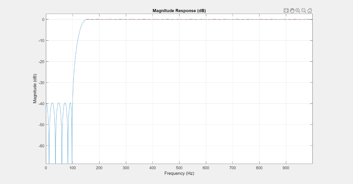
Zoom into the stopband of the highpass filter to observe that the amplitude is zero at the specified 60 Hz frequency point:
hfvt.MagnitudeDisplay = 'Magnitude';
Single-Band vs. Multi-Band IIR Designs
As in the FIR case, IIR design problems where a transition band cannot be easily identified are best resolved with a single (full) band specification approach. As an example, model the optical absorption of a gas (atomic Rubidium87 vapor):
Nb = 12;
Na = 10;
F = linspace(0,1,100);
As = ones(1,100)-F*0.2;
Absorb = [ones(1,30),(1-0.6*bohmanwin(10))',...
    ones(1,5), (1-0.5*bohmanwin(8))',ones(1,47)];
A = As.*Absorb;
d = fdesign.arbmag('Nb,Na,F,A',Nb,Na,F,A);
W = [ones(1,30) ones(1,10)*.2 ones(1,60)];
Hd = design(d, 'iirlpnorm', 'Weights', W, 'Norm', 2, 'DensityFactor',30,...
    'SystemObject',true);
fvtool(Hd, 'MagnitudeDisplay','Magnitude (dB)', ...
    'NormalizedFrequency','On');

In other cases where constraints can be relaxed in one or more transition bands, the multi-band approach provides the same benefits as in the FIR case (namely better passband and stopband characteristics). The following example illustrates these differences by modeling a Rayleigh fading wireless communications channel:
Nb = 4;
Na = 6;
F = [0:0.01:0.4 .45 1];
A = [1.0./(1-(F(1:end-2)./0.42).^2).^0.25 0 0];
d = fdesign.arbmag('Nb,Na,F,A',Nb,Na,F,A); % single-band design
Hd1 = design(d,'iirlpnorm','SystemObject',true);

B = 2;
F1 = F(1:end-2);          % Passband
F2 = F(end-1:end);        % Stopband
% F(end-2:end-1)=[.4 .45] % Transition band
A1 = A(1:end-2);
A2 = A(end-1:end);
d = fdesign.arbmag('Nb,Na,B,F,A',Nb,Na,B,F1,A1,F2,A2); % multi-band design
Hd2 = design(d,'iirlpnorm','SystemObject',true);
hfvt = fvtool(Hd1,Hd2);
legend(hfvt, 'Single-Band Design', 'Multi-Band Design');

You can also select a web site from the following list:
Americas
- América Latina (Español)
- Canada (English)
- United States (English)
Europe
- Belgium (English)
- Denmark (English)
- Deutschland (Deutsch)
- España (Español)
- Finland (English)
- France (Français)
- Ireland (English)
- Italia (Italiano)
- Luxembourg (English)
- Netherlands (English)
- Norway (English)
- Österreich (Deutsch)
- Portugal (English)
- Sweden (English)
- Switzerland
- United Kingdom (English)