Generate AUTOSAR C Code for Deep Learning Model

R2026b

This example shows how to generate AUTOSAR Classic C code from a Simulink® model that contains a trained deep neural network.

The deep neural network used in this example is trained on battery state of charge (BSOC) estimation. BSOC is the level of charge of an electric battery relative to its capacity, measured as a percentage.

This example is related to a series of examples that take you through a battery state of charge estimation workflow. For more information about the full workflow, see Battery State of Charge Estimation Using Deep Learning. For more information about the AUTOSAR standard, see What Is AUTOSAR? (AUTOSAR Blockset).

Load Trained Network

This example uses a pretrained network that has been trained to predict BSOC when provided inputs for temperature, voltage, and current. The network has been trained on data taken at four different ambient temperatures: -10°C, 0°C, 10°C, and 25°C. Load the network from the file pretrainedBSOCNetworkCompressed.mat.

For more information about training and compressing this network, see these examples:

• Train Deep Learning Network for Battery State of Charge Estimation

• Compress Deep Learning Network for Battery State of Charge Estimation

if ~exist("recurrentNet","var")
    load("pretrainedBSOCNetworkCompressed.mat");
end

Open Simulink Model

Open the model BatterySOCEstimationDeepLearning. The model contains a subsystem AI component. In this example, the AI component is a trained long short-term memory (LSTM) network that takes temperature, voltage, and current as inputs to predict BSOC.

open_system("BatterySOCEstimationDeepLearning");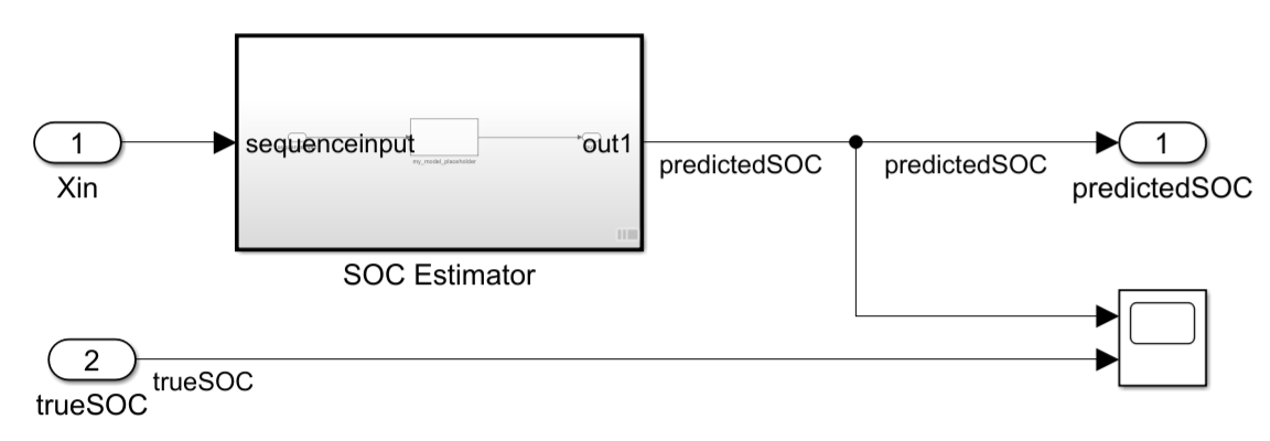

Configure Model for the AUTOSAR Classic Platform and Generate Code

Prepare held-out test data, that is, data that the AI component of the Simulink model has not seen during training. It is a best practice to use held-out test data to verify the generated code. To prepare the data, use the prepareSimulinkBSOCTestData function. prepareSimulinkBSOCTestData, which is attached to this example as a supporting function, normalizes the test data and formats it as a Dataset object, which is the format that the Simulink model expects as external input.

[steps,Ts,ds] = prepareSimulinkBSOCTestData;
set_param("BatterySOCEstimationDeepLearning", ...
    StopTime="steps", ...
    LoadExternalInput="on", ...
    ExternalInput="ds", ...
    FixedStep="Ts")

To generate AUTOSAR Classic C code, first map the model to an AUTOSAR Classic software component. To create an AUTOSAR software component mapping, set the system target file to autosar.tlc and use the autosar.api.create function.

set_param("BatterySOCEstimationDeepLearning","SystemTargetFile","autosar.tlc");
autosar.api.create("BatterySOCEstimationDeepLearning");

The autosar.api.create function creates a default Simulink-to-AUTOSAR mapping for the model and stores this mapping information in the AUTOSAR Dictionary. The software automatically maps Simulink elements to AUTOSAR interfaces, ports, and elements:

• Root-level inputs are mapped to AUTOSAR ReceiverPort elements.

• Root-level outputs are mapped to AUTOSAR SenderPort elements.

• Algorithms that use the same rate in the Simulink model are mapped to AUTOSAR runnables.

AUTOSAR receiver and sender ports are associated with AUTOSAR sender-receiver interfaces. These interfaces describe the data types and dimensions of the root-level inputs and outputs of the model. In this example, these AUTOSAR interfaces also contain information regarding the data format of the input and output layers of the deep neural network. The exported AUTOSAR XML (ARXML) file includes only internal data that is at the top level of the model.

To expose AUTOSAR internal data in ARXML descriptions, configure the model for multi-instance code generation and set the internal data packaging configuration to ArTypedPerInstanceMemory.

First, set the configuration parameter Code interface packaging to Reusable function.

set_param("BatterySOCEstimationDeepLearning","CodeInterfacePackaging","Reusable function");

Then set the internal data packaging for the model to ArTypedPerInstanceMemory.

slMapping = autosar.api.getSimulinkMapping("BatterySOCEstimationDeepLearning");
setInternalDataPackaging(slMapping, "ArTypedPerInstanceMemory");

Generate AUTOSAR code and export an ARXML file for the model by using the slbuild function.

evalc('slbuild("BatterySOCEstimationDeepLearning")');

Inspect the exported ARXML file BatterySOCEstimationDeepLearning_component.arxml. The file contains descriptions of the software component's internal behavior.

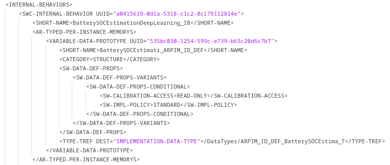
Verify Generated AUTOSAR C Code with SIL Simulations

A software-in-the-loop (SIL) simulation generates and builds code from a Simulink model and then, as a separate process on your computer, executes the built application. You can test the numerical equivalence of your model and the generated code by comparing normal simulation results with SIL simulation results. During a SIL simulation, you can collect code-coverage and execution-time metrics for the generated code.

Verify the numerical equivalence of the generated AUTOSAR code by running a SIL test. The SIL simulation compiles and executes the generated C code and then validates it against the normal Simulink simulation results.

normal_sim_output = sim("BatterySOCEstimationDeepLearning",SimulationMode="Normal");
evalc('sil_sim_output = sim("BatterySOCEstimationDeepLearning",SimulationMode="Software-in-the-loop (SIL)")');

Extract the predicted BSOC values from the normal and SIL simulation results.

time = normal_sim_output.yout{1}.Values.Time;
yout_normal = normal_sim_output.yout{1}.Values.Data;
yout_sil = sil_sim_output.yout{1}.Values.Data;

normal_predictedsoc = squeeze(yout_normal);
sil_predictedsoc = squeeze(yout_sil);

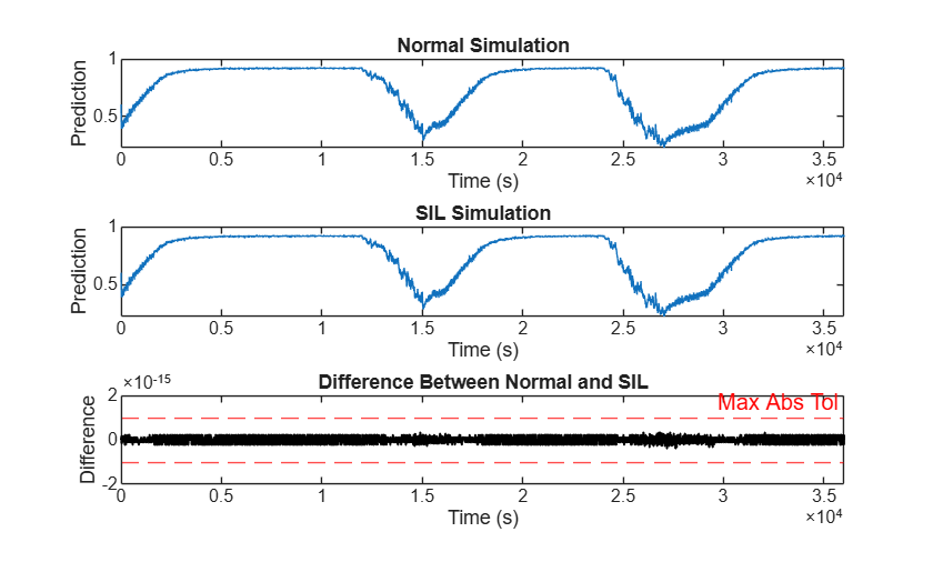
Set an absolute tolerance for the allowable difference between the predicted BSOC signals from the normal and SIL simulation results. Choose a value that meets the application requirements for numerical differences between the simulation and generated code. For this example, set the tolerance to 1e-15.

absTol = 1e-15;

Plot and compare the results. A difference within the defined tolerance range confirms numerical equivalence of the generated code and the model.

figure

subplot(3,1,1)
plot(time,normal_predictedsoc)
xlabel("Time (s)")
ylabel("Prediction")
xlim([0, steps])
title("Normal Simulation")

subplot(3,1,2)
plot(time,sil_predictedsoc)
xlabel("Time (s)")
ylabel("Prediction")
xlim([0, steps])
title("SIL Simulation")

subplot(3,1,3)
soc_diff = normal_predictedsoc - sil_predictedsoc;
plot(time,soc_diff,"k",LineWidth=1)
xlabel("Time (s)")
ylabel("Difference")
title("Difference Between Normal and SIL")

hold on
yline(absTol,"r--","Max Abs Tol")
yline(-absTol,"r--")
ylim([-2e-15, 2e-15])
xlim([0, steps])

Visualize the differences in a histogram.

figure
histogram(normal_predictedsoc - sil_predictedsoc);
xlabel("Difference")
ylabel("Frequency")
title("Normal and SIL Differences")

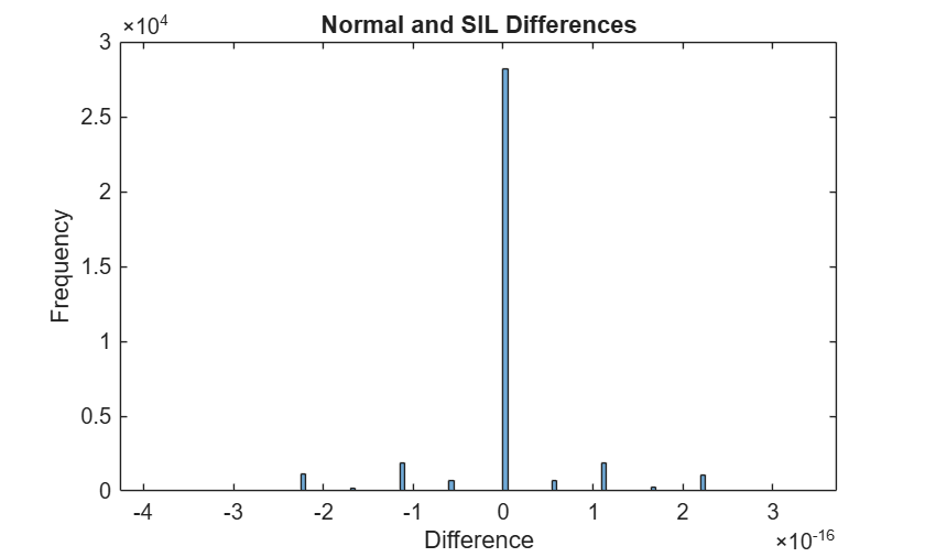
The SIL verification confirms the generated code is numerically equivalent to the model. As an additional step, evaluate the accuracy of the model predictions on the test data to confirm that the network produces reliable results.

First, extract the true SOC values from the input data set.

trueSOC = squeeze(getElement(ds,2).Data);

Because the simulation runs one step beyond the input data, trim the simulation outputs to match the true SOC length.

nSteps = numel(trueSOC);
time = time(1:nSteps);
normal_predictedsoc = normal_predictedsoc(1:nSteps);

Plot the predicted BSOC against the true BSOC.

figure
subplot(2,1,1)
plot(time,normal_predictedsoc)

hold on
plot(time,trueSOC)
hold off

legend("Predicted BSOC","True BSOC")
title("Predicted vs True BSOC")
xlabel("Time (s)")
ylabel("State of Charge")

subplot(2,1,2)
plot(time,normal_predictedsoc - trueSOC)
title("Prediction Error (Predicted - True)")
xlabel("Time (s)")
ylabel("\DeltaBSOC")

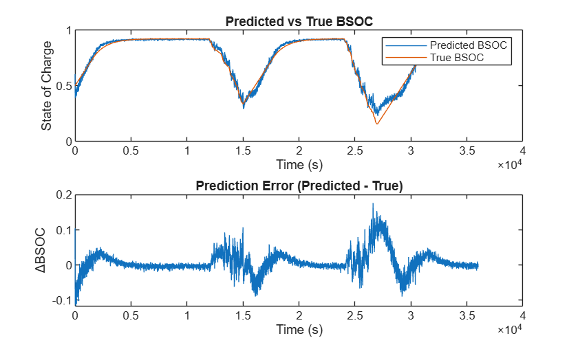
Visualize the prediction errors in a histogram.

figure
histogram(normal_predictedsoc - trueSOC);
xlabel("Error")
ylabel("Frequency")
title("Prediction Errors")

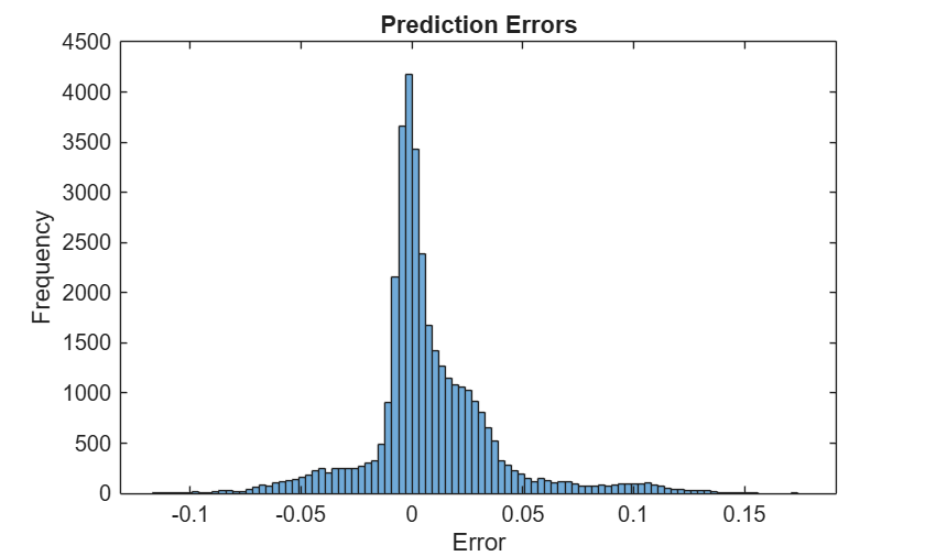
Error values close to zero indicate a good model fit.

Calculate the root mean squared error (RMSE) value.

err = rmse(normal_predictedsoc,trueSOC)

err = 
0.0307

As a next step, you can deploy the generated code to an embedded target. For an example that shows how to deploy this network to an STM32 microcontroller, see Deploy Code for Battery State of Charge Estimation Using Deep Learning.