Main Content

ModalTruncation

Modal truncation model order reduction specification

Since R2023b

    Description

    The ModalTruncation object stores model order reduction (MOR) specifications for the modal truncation of ordinary (nonsparse) linear time-invariant (LTI) models.

    Modal truncation is based on the modal decomposition

    G(s)=D+k=1ncGk(s).

    Each modal component in Gk(s) is associated with a single real pole, a pair of complex conjugate poles, or a cluster of repeated real or complex poles. Here, a cluster means that the poles of Gk(s), while not identical, cannot be separated in a numerically safe way. The software obtains the modal decomposition by block diagonalization of A or (A,E).

    Creation

    The reducespec function creates a modal truncation model order reduction object when you use this syntax.

    R = reducespec(sys,"modal")

    Here, sys is any nonsparse LTI model. The workflow uses this object to set up MOR tasks and store results. For the full workflow, see Task-Based Model Order Reduction Workflow.

    Properties

    expand all

    This property is read-only.

    Average mode (pole) value in the modal component Gk, returned as a vector of length nc-by-1, where nc is the number of modal components.

    • When R.Options.ModeOnly = true, Mode contains only the poles of sys.

    • When R.Options.ModeOnly = false, Mode has one entry for each modal component Gk(s), which corresponds to the average pole location in Gk(s). For clusters associated with complex pairs of eigenvalues, this is the average of the eigenvalues with positive real part.

    This property is read-only.

    Damping ratio of average poles in the modal component Gk(s), returned as a vector of length nc-by-1, where nc is the number of modal components.

    This property is read-only.

    Natural frequency of average poles in the modal component Gk(s), returned as a vector of length nc-by-1, where nc is the number of modal components.

    This property is read-only.

    Modal components Gk(s), returned as an nc-by-1 array of state-space models, where nc is the number of modal components.

    This property is read-only.

    Normalized DC contribution of modal components, returned as a vector of length nc-by-1, where nc is the number of modal components.

    These values are the DC gains of each modal component Gk(s) divided by the DC gain of the overall system. In some cases, the normalized DC contributions can exceed one if there are modal cancellations near DC (the overall DC gain is smaller than the sum of the DC contributions of each modal component).

    This property is read-only.

    Left-side matrix of block-diagonalizing transformation, returned as a matrix of size N-by-N, where N is the number of states in the original model sys.

    The modal truncation algorithm transforms the state-space realization (A, B, C, D, E) of sys to block diagonal matrices (Am, Bm, Cm, Dm, Em) given by:

    • For explicit state-space models

      Am=TLTATR,Bm=TLTB,Cm=CTR,Dm=D,TLTTR=I

    • For descriptor state-space models

      Am=TLTATR,Bm=TLTB,Cm=CTR,Dm=D,Em=TLTETR

    This property is read-only.

    Right-side matrix of block-diagonalizing transformation, returned as a matrix of size N-by-N, where N is the number of states in the original model sys.

    The modal truncation algorithm transforms the state-space realization (A, B, C, D, E) of a model to block diagonal matrices (Ak, Bk, Ck, Dk, Ek) given by:

    • For explicit state-space models

      Am=TLTATR,Bm=TLTB,Cm=CTR,Dm=D,TLTTR=I

    • For descriptor state-space models

      Am=TLTATR,Bm=TLTB,Cm=CTR,Dm=D,Em=TLTETR

    Options for modal truncation of LTI models, specified as a ModalTruncationOptions object. Use dot notation to configure options for R. For example R.Options.ModeOnly = true.

    For more information about available options, see ModalTruncationOptions..

    Object Functions

    processRun model order reduction algorithm
    view (modal)Plot mode information when using modal truncation method
    getrom (modal)Obtain reduced-order models when using modal truncation method

    Examples

    collapse all

    This example shows how to obtain a reduced-order model for a linear time-invariant (LTI) model using the modal truncation method. In this example, you reduce a high-order model with a focus on the dynamics in a particular frequency range and damping.

    Load a model and examine its frequency response.

    load('highOrderModel.mat','G')
    bodeplot(G)

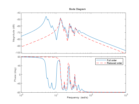
    G is a 48th-order model with several large peak regions around 5.2 rad/s, 13.5 rad/s, and 24.5 rad/s, and smaller peaks scattered across many frequencies.

    Create a model order reduction task.

    R = reducespec(G,"modal");
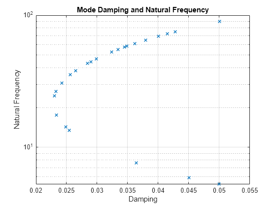
    view(R,"damp")

    Suppose that for your application you are only interested in the dynamics between 10 rad/s and 40 rad/s with damping less than 0.04. Focus the model reduction on the region of interest to obtain a good match with a low-order approximation.

    rsys = getrom(R,Frequency=[10,40],Damping=[0.022 0.04]);
    opt = bodeoptions;
    opt.PhaseMatching = "on";
    bodeplot(G,rsys,"r--",opt)
    legend("Full order","Reduced order")

    The reduced-order model provides a good approximation for the specified targets.

    Algorithms

    • When R.Options.ModeOnly is set to true, the software just transforms A or (A,E) to Schur or QZ form.

    • When R.Options.ModeOnly is set to false, the software computes the full modal decomposition G(s)=D+k=1ncGk(s)..

    In both cases, once you decide which modes to keep and which modes to discard, the algorithm obtains the decomposition G(s) = G1(s) + G2(s) + D, where G1(s) contains the desired modes. Then, based on the specified method, getrom returns the reduced-order model as follows.

    • "truncate"Gr(s) = G1(s) + D

    • "matchDC"Gr(s) = G1(s) + D + G2(0)

    Version History

    Introduced in R2023b