Interactively Estimate Plant Parameters from Response Data

R2026b

This example shows how to use PID Tuner to fit a linear model to measured SISO response data.

If you have System Identification Toolbox™ software, you can use PID Tuner to estimate the parameters of a linear plant model based on time-domain response data measured from your system. PID Tuner then tunes a PID controller for the resulting estimated model. PID Tuner gives you several techniques to graphically, manually, or automatically adjust the estimated model to match your response data. This example illustrates some of those techniques.

In this example, you load measured response data from a data file into the MATLAB^® workspace you represent the plant as an LTI model. For information about generating simulated data from a Simulink^® model, see Interactively Estimate Plant from Measured or Simulated Response Data (Simulink Control Design).

Load Measured Response Data

Open Live Script

Load the measured response data for this example into the MATLAB® workspace.

load PIDPlantMeasuredIOData

When you import response data, PID Tuner assumes that your measured data represents a plant connected to the PID controller in a negative-feedback loop. In other words, PID Tuner assumes the following structure for your system. PID Tuner assumes that you injected a step signal at the plant input u and measured the system response at y, as shown.

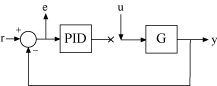
The sample data file for this example, contains three variables, each of which is a 501-by-1 array. inputu is the unit step function injected at u to obtain the response data. outputy is the measured response of the system at y. The time vector t, runs from 0 to 50 s with a 0.1 s sample time. Comparing inputu to t shows that the step occurs at t = 5 s.

You can import response data stored as a numeric array (as in this example), a timeseries object, or an iddata object.

Import Response Data for Identification

Open PID Tuner.
```
pidTuner(tf(1),'PI')
```
In PID Tuner, in the Plant menu, select Identify New Plant.
In the Plant Identification tab, click Get I/O data and select Step Response. This action opens the Import Step Response dialog box.
Enter information about the response data. The output signal is the measured system response, outputy. The input step signal is parametrized as shown in the diagram in the dialog box. Here, enter 5 for the Onset Lag, and 0.1 for Sample Time. Then, click Import.
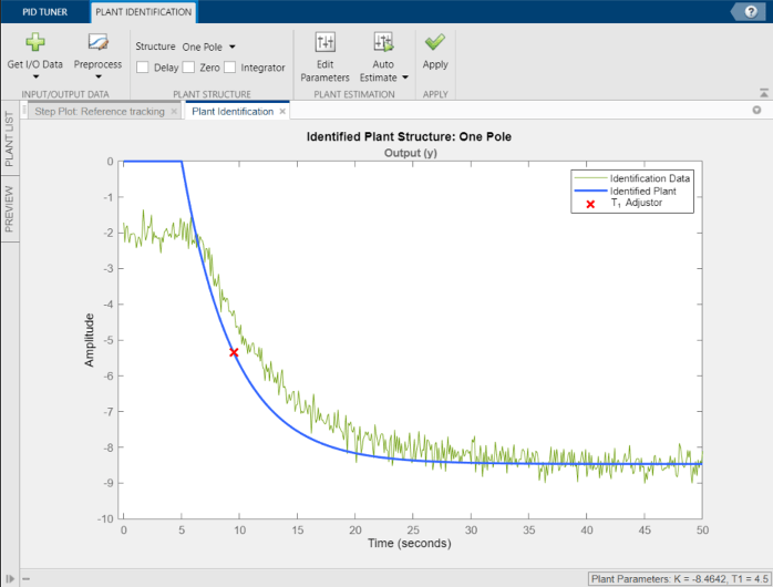
The Plant Identification plot displays the response data and the response of an initial estimated plant.

Preprocess Data

Depending on the quality and features of your response data, you might want to perform some preprocessing on the data to improve the estimated plant results. PID Tuner provides several options for preprocessing response data, such as removing offsets, filtering, or extracting a subset of the data. In this example, the response data has an offset. It is important for good identification results to remove data offsets. Use the Preprocess menu to do so. (For information about other data preprocessing options, see Preprocess Data.)

On the Plant Identification tab, click Preprocess and select Remove Offset. The Remove Offset tab opens, displaying time plots of the response data and corresponding input signal.
Select Remove offset from signal and choose the response, Output (y). In the Offset to remove text box, specify a value of –2. You can also select the signal initial value or signal mean, or enter a numerical value. The plot updates with an additional trace showing the signal with the offset applied.
Click Apply to save the change to the signal. Click Close Remove Offset to return to the Plant Identification tab.
PID Tuner automatically adjusts the plant parameters to create a new initial guess for the plant based on the preprocessed response signal.

Adjust Plant Structure and Parameters

PID Tuner allows you to specify a plant structure, such as One Pole, Underdamped Pair, or State-Space Model. In the Structure menu, choose the plant structure that best matches your response. You can also add a transport delay, a zero, or an integrator to your plant. For this example, the one-pole structure gives the qualitatively correct response. You can make further adjustments to the plant structure and parameter values to make the estimated system’s response a better match to the measured response data.

PID Tuner gives you several ways to adjust the plant parameters:

Graphically adjust the response of the estimated system by dragging the adjustors on the plot. In this example, drag the red x to adjust the estimated plant time constant. PID Tuner recalculates system parameters as you do so. As you change the estimated system’s response, it becomes apparent that there is some time delay between the application of the step input at t = 5 s, and the response of the system to that step input.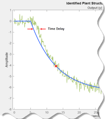
To add a transport delay to the estimated plant model, in the Plant Structure section, check Delay. A vertical line appears on the plot, indicating the current value of the delay. Drag the line left or right to change the delay, and make further adjustments to the system response by dragging the red x.
Adjust the numerical values of system parameters such as gains, time constants, and time delays. To numerically adjust the values of system parameters, click Edit Parameters.
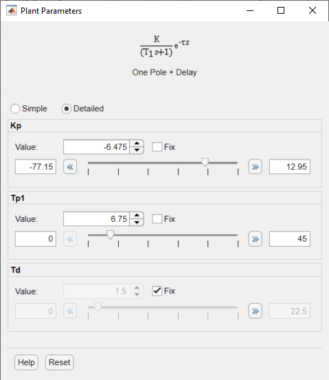
Suppose that you know from an independent measurement that the transport delay in your system is 1.5 seconds. In the Plant Parameters dialog box, enter 1.5 for τ. Select Fix to fix the parameter value. When you select Fix for a parameter, neither graphical nor automatic adjustments to the estimated plant model affect that parameter value.
Automatically optimize the system parameters to match the measured response data. Click Auto Estimate to update the estimated system parameters using the current values as an initial guess.

You can continue to iterate using any of these methods to adjust plant structure and parameter values until the response of the estimated system adequately matches the measured response.

Estimation Options

When you automatically estimate structure parameters, you can specify options for the fit frequency range, initial conditions, and iteration options.

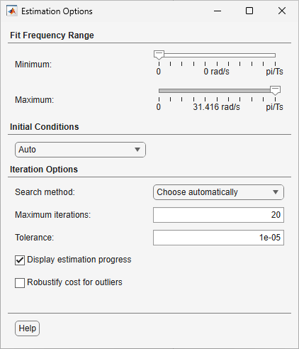
By default, the software attempts to fit the data across the entire frequency range from 0 to the Nyquist frequency. You can adjust the fit frequency range by adjusting the Minimum and Maximum sliders.

You can specify how the software handles the plant initial conditions during estimation using the Initial Conditions drop-down list.

Auto — By default, the software chooses a method for handling initial conditions based on the estimation data. If the initial states have negligible effect on the prediction errors, the initial states are set to zero to optimize algorithm performance.
Zero — Set all initial state values to zero.
Estimate — Treat initial state values as a vector of independent estimation parameters. The software estimates these values from the data.
Backcast — Estimate the initial condition using the best least squares fit.

You can configure the plant estimation algorithm using the options in this table.

Option	Description
Search method	Search method used by iterative search algorithm to find parameter values that optimally fit the response data. `Choose Automatically` — (Default) The software chooses the optimization method automatically. `Gauss-Newton` — Gauss-Newton direction based linear search scheme. `Adaptive Gauss-Newton` — Gauss-Newton direction with an adaptive cutoff of singular values. `Levenberg-Marquardt` — Traditional Levenberg-Marquardt direction-based linear search. `Gradient Search` — Steepest descent direction-based linear search. `Trust-Region Reflective Newton` — Nonlinear least-squares method (requires Optimization Toolbox™ software). `Pattern Search` — Solver for nonlinearities without well-defined gradients (requires Global Optimization Toolbox software). `Sequential Quadratic Programming Search` — Sequential quadratic programming algorithm that satisfies bounds at all iterations and can recover from `NaN` or `Inf` results (requires Optimization Toolbox software). `Interior Point` — Large-scale algorithm that satisfies bounds at all iterations and can recover from `NaN` or `Inf` results (requires Optimization Toolbox software).
Maximum iterations	Maximum number of iterations to perform if the tolerance is not satisfied.
Tolerance	Iterations terminate when the expected improvement in the fit criterion is less than this value (in percent).
Display estimation progress	Select this option to see a display of the estimation status at each iteration.
Robustify cost for outliers	When you select this option, residuals in the fit that are larger than a scaling value times the estimated standard deviation carry a linear rather than quadratic weight. When you clear this option, a pure quadratic criterion is used instead.

Save Plant and Tune PID Controller

When you are satisfied with the fit, click Apply. Doing so saves the estimated plant, Plant1, to the PID Tuner workspace. PID Tuner automatically designs a PI controller for Plant1 and, in the Step Plot: Reference Tracking plot, displays a new closed-loop response. The Plant List table reflects that Plant1 is selected for the current controller design.

Tip

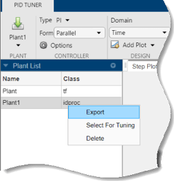
To examine variables stored in the PID Tuner workspace, view the Plant List.

You can now use the PID Tuner tools to refine the controller design for the estimated plant and examine tuned system responses.

You can also export the identified plant from the PID Tuner workspace to the MATLAB workspace for further analysis. On the PID Tuner tab, click Export. Check the plant model you want to export to the MATLAB workspace. For this example, export Plant1, the plant you identified from response data. You can also export the tuned PID controller. Click OK. The models you selected are saved to the MATLAB workspace.

Identified plant models are saved as identified LTI models, such as idproc (System Identification Toolbox) or idss (System Identification Toolbox).