Optimization of Antenna Array Elements Using Antenna Array Designer App
This example demonstrates how to maximize the gain of 2-by-2 patch array antenna elements using a surrogate model-assisted differential evolution for antenna synthesis (SADEA) optimizer. The design and analysis are performed at 2.4 GHz.
Open Antenna Array Designer App
Enter antennaArrayDesigner at the MATLAB® command prompt to open the app.
The command opens a blank canvas. In the blank canvas, click New.

Design Rectangular Microstrip Patch Array
In the New tab, select Rectangular from Array Gallery. Select Antenna Gallery > Microstrip under Patch family.
Select No Backing under Backing Structure Gallery section.
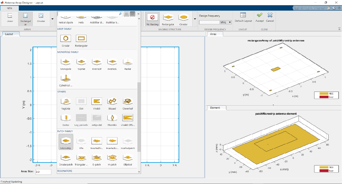
Set the Design Frequency value to 2.4 GHz. Set Array size to 2,2.
To analyze this antenna array, click Accept.

Plot 3-D Radiation Pattern
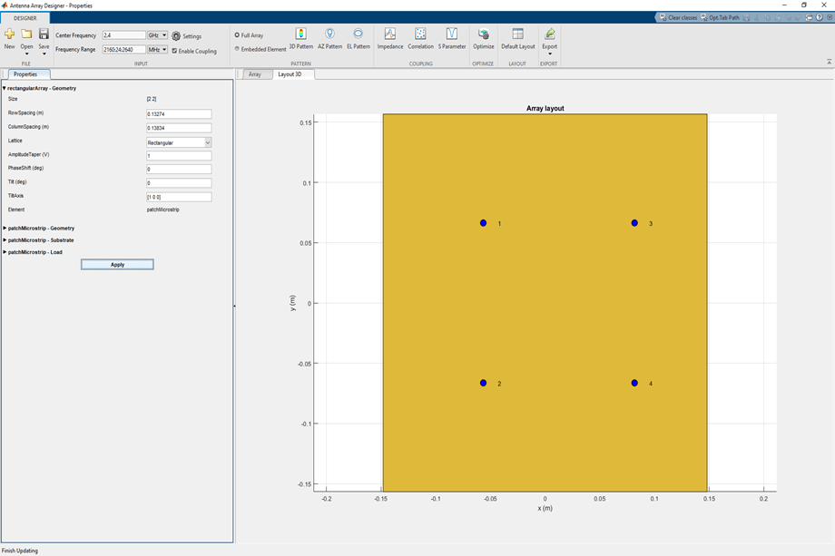
Observe the rectangular array of microstrip patch antenna and the layout of the geometry at 2.4 GHz in the Array and Layout 3D figure tabs.
In the toolstrip, under the PATTERN section, click 3-D Pattern to visualize the radiation pattern. The maximum gain of array is 14.8 dBi.

Plot 2-D Elevation Pattern to Measure Front to Back Lobe Ratio
In the toolstrip, under the PATTERN section, click EL Pattern to visualize the front to back (F/B) lobe ratio. Right click on the plot and select Measurements > Antenna Metrices. A dialog box appears with the message**: Existing markers will be removed.** Select Remove.
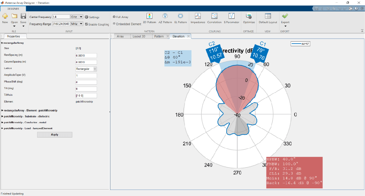
The F/B(dB) is 31.2 dB.
Define Optimization Goal
To optimize an antenna array using the Antenna Array Designer App, these inputs are required:
Objective function: The main goal of the optimization. The objective function evaluates the analysis function and minimizes or maximizes the output of the function.
Design variables: The input variables that have to be optimized to achieve the objective function under certain constraints. These variables are changed by the optimizer within a preset range of values called the bounds of the variables.
Constraints: The conditions under analysis that must be satisfied. The constraints are optional. If there are multiple constraints, then the user can prioritize the constraints using the % Weight parameter.
Other inputs: These inputs might include number of iterations, center frequency, and frequency range at which the analysis is performed.
Optimization Goal: To maximize gain of the rectangular patch array antenna using the F/B lobe ratio as a constraint to maintain the desired direction of the main lobe.
In this example, inputs are:
Objective function : Maximize Gain (dBi).
Design variables : RowSpacing, ColumnSpacing, GroundPlaneLength and GroundPlaneWidth.
Constraints :F/B lobe ratio (dB).
Set Optimizer
To optimize the rectangular patch array antenna, click Optimize under Optimize section.
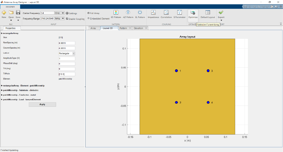
The optimizer supports several objective functions. This example uses maximizing gain as an objective function.
In this example, the optimizer can take up to seven hours to converge. To meet the objectives, these machine configurations are preferred:
Processor: Intel ® Xeon ® CPU E5-1650 v4 @3.60GHz.
RAM: 64GB.
System type: 64-bit operating system.
Set Objective Function
To select the objective function, select Maximize Gain.
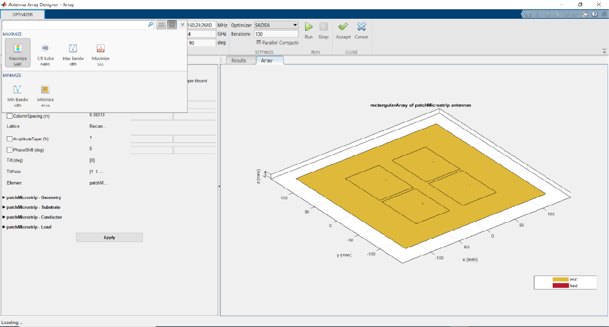
Set Design Variables
To set design variables, select the Design Variables tab. Select the checkboxes to select the design variables. These variables are optimized to obtain maximum gain of the antenna.

In this example, select the check boxes corresponding to RowSpacing and ColoumnSpacing under rectangularArray-Geometry and GroundPlaneLength and GroundPlaneWidth under patchMicrostrip -Geometry.
Design variables are set based on the values shown in the table.

Click Apply to set the variables.
Set Constraints to Optimization Goal
Choose the Constraint Function under Constraint tab.
To set constraints, choose F/B Lobe Ratio (dB) as the Constraint Function from Constraint pane select **‘>’**operator under sign and set Value as 31.

Click Apply to accept the Constraints.
To input the number of iterations, in Settings section, set Iterations to 200 and select Parallel Computing if you have Parallel Computing Toolbox™.
Run SADEA Optimization
To start optimization, click Run.
The SADEA algorithm contains two stages
Building model
Optimization
In the building model stage, the optimizer makes a surrogate model from the design space, specified objective, and the constraints function. In the design space analysis are performed on sample points.
As a result, the X-axis shows the number of samples, and the Y-axis shows the value of the analysis function value at that sample. The bottom left side of the app window shows the current sample value, and the bottom right side of the app window shows the design variables. The optimizer takes an appropriate number of samples to build the model. After the model is built, the optimizer starts running iterations.
In the optimization stage, the X-axis shows the number of iterations, and the Y-axis shows the objective function values. From the plots shown on the optimizing stage, you can understand the trend of convergence.

Note: The objective and the constraint plots show fewer deviations. After the 170th iteration, the two plots converge.
Optimized 3-D Pattern and Front to Back Lobe Ratio
Once optimization is complete, click Accept. Click Apply to analyze the 3-D and 2-D patterns.
To observe the 3-D radiation pattern of the optimized antenna, click 3D Pattern in the Pattern section. The maximum directivity is observed as 16.8 dBi.

Click EL Pattern in Pattern section to observe the F/B lobe ratio. The optimized antenna F/B lobe ratio is 31.4 dB.

The table shows a comparison of the results.

See Also
Maximizing Gain and Improving Impedance Bandwidth of E-Patch Antenna