Design and Analyze Microstrip Patch Antenna with Frequency-Dependent Dielectric Models
R2026bThis example shows how to design a microstrip patch antenna at 3.5 GHz using Antenna Toolbox and analyze it using constant, Djordjevic-Sarkar, and Table-Driven frequency-dependent dielectric models. The design function automatically computes optimal patch dimensions, feed offset, and ground plane size for the specified substrate and frequency. This eliminates the need for manual analytical calculations.
Define Design Parameters
Specify the operating frequency and substrate geometry. The microstrip patch antenna targets 5G applications at 3.5 GHz. Choose FR4 as the substrate with a standard PCB thickness of 1.6 mm.
f_design = 3.5e9;
h_sub = 1.6e-3;
Create Dielectric Substrates Using Three Frequency Models
The dielectric object supports multiple frequency models that represent material dispersion with varying levels of fidelity. Each model serves a different design scenario:
Constant — Frequency-independent; suitable for narrowband designs
Djordjevic-Sarkar — Causal wideband model from a single measurement point
Table-Driven — Uses measured data at multiple frequencies with rational fitting
Model 1: Constant Frequency Model
The Constant model assigns fixed values of relative permittivity and loss tangent across all frequencies. This is the default behavior and works well for narrowband designs where the substrate properties do not change significantly over the operating bandwidth. Here the built-in FR4 material catalog entry is used with its FrequencyModel set to Constant.
d_constant = dielectric("FR4");
d_constant.FrequencyModel = "Constant";
Model 2: Djordjevic-Sarkar Frequency Model
The Djordjevic-Sarkar model provides a causal, frequency-dependent representation based on a wideband Debye relaxation formulation. It extrapolates material properties over a wide frequency range from permittivity and loss tangent measured at a single reference frequency (here 1 GHz). This model ensures causality, meaning the Kramers-Kronig relations are satisfied.
d_djordjevic = dielectric("FR4");
d_djordjevic.FrequencyModel = "DjordjevicSarkar";
Model 3: Table-Driven Frequency Model
The Table-Driven model uses measured or computed dielectric data at multiple frequency points. A rational function is fitted internally to interpolate and extrapolate between data points. When measured characterization data is available (for example, from split-post dielectric resonator or transmission line methods), this is the highest-fidelity model.
The input data must satisfy causality constraints: permittivity must decrease monotonically while loss tangent increases monotonically with frequency, and variations must be small.
TableDrivenData=load("TableDrivenData.mat");
TableData = TableDrivenData.TableData;
Create Table-Driven Dielectric for Material Property Evaluation
Use the entire multi-frequency data set to create a dielectric object and evaluate material properties across the band. Assign the frequency, permittivity, and loss tangent vectors from the table, and set the substrate thickness is to 1.6 mm.
d_tabledriven_eval = dielectric;
d_tabledriven_eval.Name = "CustomDielectric";
d_tabledriven_eval.FrequencyModel = "TableDriven";
d_tabledriven_eval.Frequency = TableData{:,1};
d_tabledriven_eval.EpsilonR = TableData{:,2};
d_tabledriven_eval.LossTangent = TableData{:,3};
d_tabledriven_eval.Thickness = h_sub
d_tabledriven_eval =
  dielectric with properties:

              Name: 'CustomDielectric'
          EpsilonR: [15×1 double]
       LossTangent: [15×1 double]
         Thickness: 0.0016
         Frequency: [15×1 double]
    FrequencyModel: 'TableDriven'

For more materials see catalog
Verify Material Properties Over Frequency
Use the getMaterialProperties function to inspect how each model represents the substrate across the analysis band from 1 GHz to 10 GHz. This verification step confirms that the frequency-dependent models produce physically meaningful results before proceeding with antenna analysis.
freq_range = linspace(1e9, 10e9, 200);
[epsr_const, loss_const] = getMaterialProperties(d_constant, freq_range);
[epsr_djord, loss_djord] = getMaterialProperties(d_djordjevic, freq_range);
[epsr_table, loss_table] = getMaterialProperties(d_tabledriven_eval, freq_range);
Relative Permittivity Comparison
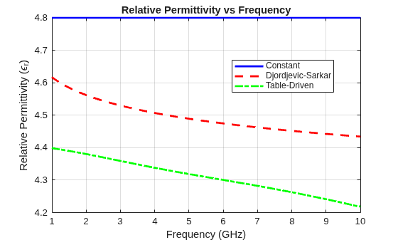
The Constant model remains flat, whereas the Djordjevic-Sarkar and Table-Driven models show the expected monotonic decrease in permittivity with frequency.
plot(freq_range/1e9, epsr_const, "b-", LineWidth=2);
hold on;
plot(freq_range/1e9, epsr_djord, "r--", LineWidth=2);
plot(freq_range/1e9, epsr_table, "g-.", LineWidth=2);
hold off;
grid on;
xlabel("Frequency (GHz)");
ylabel("Relative Permittivity (\epsilon_r)");
title("Relative Permittivity vs Frequency");
legend("Constant","Djordjevic-Sarkar","Table-Driven",Location="best");
xlim([1 10]);
Loss Tangent Comparison
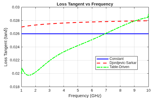
The loss tangent increases monotonically with frequency for the dispersive models, capturing the realistic behavior of FR4 at higher frequencies.
plot(freq_range/1e9, loss_const, "b-", LineWidth=2);
hold on;
plot(freq_range/1e9, loss_djord, "r--", LineWidth=2);
plot(freq_range/1e9, loss_table, "g-.", LineWidth=2);
hold off;
grid on;
xlabel("Frequency (GHz)");
ylabel("Loss Tangent (tan\delta)");
title("Loss Tangent vs Frequency");
legend("Constant","Djordjevic-Sarkar","Table-Driven",Location="best");
xlim([1 10]);
Evaluate Material Properties at the Design Frequency
Compare the effective permittivity and loss tangent that each model predicts at 3.5 GHz.
[epsr_at_f_const, loss_at_f_const] = getMaterialProperties(d_constant, f_design);
[epsr_at_f_djord, loss_at_f_djord] = getMaterialProperties(d_djordjevic, f_design);
[epsr_at_f_table, loss_at_f_table] = getMaterialProperties(d_tabledriven_eval, f_design);

modelNames = {"Constant"; "Djordjevic-Sarkar"; "Table-Driven"};
epsrVals = [epsr_at_f_const; epsr_at_f_djord; epsr_at_f_table];
lossVals = [loss_at_f_const; loss_at_f_djord; loss_at_f_table];

T_material = table(modelNames, epsrVals, lossVals, ...
    'VariableNames', {'Model','Dk(3.5 GHz)','Df(3.5 GHz)'})
T_material = 3×3 table
Model Dk(3.5 GHz) Df(3.5 GHz)
_______________________ ___________ ___________
{["Constant" ]} 4.8 0.026
{["Djordjevic-Sarkar"]} 4.5175 0.027564
{["Table-Driven" ]} 4.35 0.0225
Create Patch Antennas with Different Dielectric Models
For each dielectric model, create a patchMicrostrip object with the specified substrate and height.
ant_constant = design(patchMicrostrip(Substrate=d_constant),f_design);
ant_constant.Height = h_sub
ant_constant =
  patchMicrostrip with properties:

               Length: 0.0190
                Width: 0.0244
               Height: 0.0016
            Substrate: [1×1 dielectric]
    GroundPlaneLength: 0.0391
     GroundPlaneWidth: 0.0391
    PatchCenterOffset: [0 0]
           FeedOffset: [0.0040 0]
            Conductor: [1×1 metal]
                 Tilt: 0
             TiltAxis: [1 0 0]
                 Load: [1×1 lumpedElement]
ant_djordjevic = design(patchMicrostrip(Substrate=d_constant),f_design);
ant_djordjevic.Substrate = d_djordjevic;
ant_djordjevic.Height = h_sub
ant_djordjevic =
  patchMicrostrip with properties:

               Length: 0.0190
                Width: 0.0244
               Height: 0.0016
            Substrate: [1×1 dielectric]
    GroundPlaneLength: 0.0391
     GroundPlaneWidth: 0.0391
    PatchCenterOffset: [0 0]
           FeedOffset: [0.0040 0]
            Conductor: [1×1 metal]
                 Tilt: 0
             TiltAxis: [1 0 0]
                 Load: [1×1 lumpedElement]
ant_tabledriven = design(patchMicrostrip(Substrate=d_constant),f_design);
ant_tabledriven.Substrate = d_tabledriven_eval;
ant_tabledriven.Height = h_sub
ant_tabledriven =
  patchMicrostrip with properties:

               Length: 0.0190
                Width: 0.0244
               Height: 0.0016
            Substrate: [1×1 dielectric]
    GroundPlaneLength: 0.0391
     GroundPlaneWidth: 0.0391
    PatchCenterOffset: [0 0]
           FeedOffset: [0.0040 0]
            Conductor: [1×1 metal]
                 Tilt: 0
             TiltAxis: [1 0 0]
                 Load: [1×1 lumpedElement]
Visualize Antenna Geometry
Display the geometry of the microstrip patch antenna. All three antennas share the same physical topology except the dielectric substrate model differs.
show(ant_constant);
title(sprintf("Microstrip Patch Antenna for %.1f GHz on FR4 (h=1.6 mm)", f_design/1e9));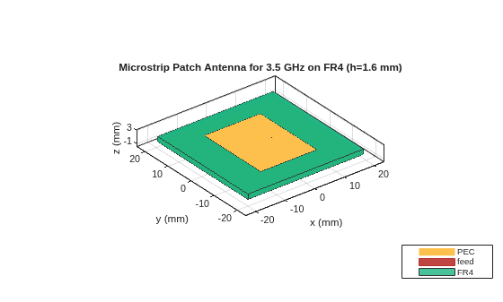
Compute S-Parameters with Frequency Sweep
Use the frequencySweep object with interpolation mode to efficiently compute S-parameters from 2.0 to 5.0 GHz with 51 frequency points.
h = frequencySweep;
h.SweepType = "interp";
h.NumFreqs = 51;
m_constant= mesh(ant_constant,MaxEdgeLength=0.012);
S_const_ext = sparameters(ant_constant, [2.0e9, 5.0e9],SweepOption=h);
m_djordjevic = mesh(ant_djordjevic,MaxEdgeLength=0.012);
S_djord_ext = sparameters(ant_djordjevic, [2.0e9, 5.0e9],SweepOption=h);
m_tabledriven= mesh(ant_tabledriven,MaxEdgeLength=0.012);
S_table_ext = sparameters(ant_tabledriven, [2.0e9, 5.0e9],SweepOption=h);
Compare Reflection Coefficients
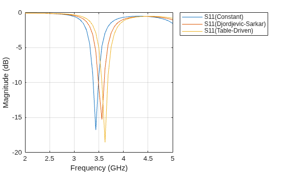
The extended sweep from 2 to 5 GHz shows the response for the dielectric models. This comparison reveals differences in resonant frequency depth and bandwidth caused by the different substrate models.
rfplot(S_const_ext)
hold on
rfplot(S_djord_ext)
rfplot(S_table_ext)
lgd = legend;
lgd.String = {"S11(Constant)", "S11(Djordjevic-Sarkar)","S11(Table-Driven)"};
3-D Radiation Pattern
Compute and display the 3-D radiation pattern at the design frequency.
pattern(ant_constant, f_design);
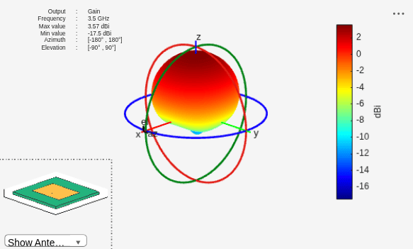
pattern(ant_djordjevic, f_design);
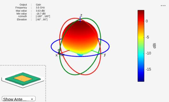
pattern(ant_tabledriven, f_design);
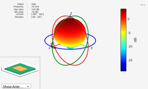
Differences among models arise because the loss tangent affects radiation efficiency and the effective permittivity influences fringing fields.
GainValues_dBi = [3.55;3.62;4.09];
T_GainVariation = table(modelNames, epsrVals, lossVals,GainValues_dBi, ...
    'VariableNames', {'Model','EpsilonR_at_3.5 GHz','LossTangent_at_3.5 GHz','GainValues(dBi)_at_3.5 GHz'})
T_GainVariation = 3×4 table
             Model             EpsilonR_at_3.5 GHz    LossTangent_at_3.5 GHz    GainValues(dBi)_at_3.5 GHz
    _______________________    ___________________    ______________________    __________________________

    {["Constant"         ]}             4.8                     0.026                      3.55
    {["Djordjevic-Sarkar"]}          4.5175                  0.027564                      3.62
    {["Table-Driven"     ]}            4.35                    0.0225                      4.09

