Antenna Designer
R2026bDesign, visualize, and analyze antennas
Description
The Antenna Designer app lets you design, visualize, and analyze antennas in the Antenna Toolbox library interactively.
Using this app, you can:
Select antennas based on general properties or antenna performance.
Select backing structures from the gallery of backing structures.
Visualize antennas based on frequency and frequency range.
Analyze antennas based on radiation pattern, polarization, and bandwidth.
Export selected and designed antennas as a variable to the MATLAB® workspace, as either script or a variable. The exported MATLAB script has two sections:
Antenna PropertiesandAntenna Analysis.Save and load an existing antenna .mat file to the app and analyze the antenna.
Optimize antennas for various analysis results under given constraints using SADEA or Surrogate optimization methods.
Note
To use Parallel Computing for
SADEAoptimizer, you need the Parallel Computing Toolbox™.
To use the Surrogate optimization algorithm, you need the Global Optimization Toolbox.

Open the Antenna Designer App
MATLAB Toolstrip: In the APPS tab, under RF AND MIXED-SIGNAL, click the Antenna Designer app icon.
MATLAB command prompt: Enter
antennaDesigner.
Examples
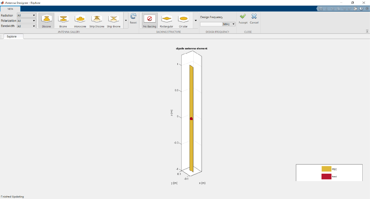
The Antenna Designer opens a blank canvas.

Select and Visualize Antenna
Click

in the canvas toolstrip to choose the antenna you want to analyze.
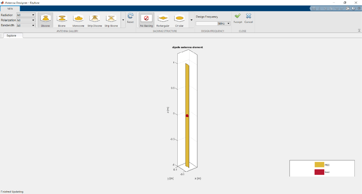
The default antenna is a dipole antenna.

You can filter the antennas based on
Radiationpattern,Polarization, andBandwidth.Using options in the BACKING STRUCTURE menu, you can add cavity and reflector type backing structures to the antenna.
You can add dielectric material as a substrate to the supported antennas using the DIELECTRIC CATALOG drop-down options. You can add predefined material, single or multiple dielectric layers, or specify a material using its dielectric property values.
You can also specify the Design Frequency of the antenna. Setting this value scales the antenna to resonate at the specified frequency. You can also tune the antenna using Antenna Properties tab during analysis.
Use Reset, to go back to default settings.
Use Accept, to analyze the antenna characteristics.
Use Cancel, to start over.
Antenna Gallery
You can choose your antennas from the ANTENNA GALLERY.

When you filter antennas based on
Radiationpattern,Polarization, orBandwidth, the antenna gallery greys out the antennas that do not belong to the chosen filter.
Back Structure Gallery
You can choose your antenna backing structures from the BACKING STRUCTURE GALLERY.

Analyze Antenna
You can estimate the memory required to solve the antenna mesh by clicking the Memory Estimate button.
You can manually mesh the antenna by changing the Meshing Mode to manual in the Analysis Settings menu, defining and saving mesh parameters, and then clicking on the Mesh button.
You can plot the Impedance and S Parameter of the antenna based on the specified Frequency Range in Hz.
You can visualize the Current distribution on the antenna based on the specified Frequency in Hz.
You can visualize the 3D Pattern, AZ Pattern, EL Pattern of the antenna based on the specified frequency. Here
AZstands for azimuth andELstands for elevation.Use Export to view your antenna in MATLAB workspace or MATLAB script.
Manually change the antenna properties using the Antenna Properties tab. In this tab, you can change the geometrical properties of the antenna, add a dielectric substrate and metal conductor parameters to the antenna, and change the value and location of the load.
Optimize Antenna
Click on Optimize to open the optimizer canvas of the antenna designer app.
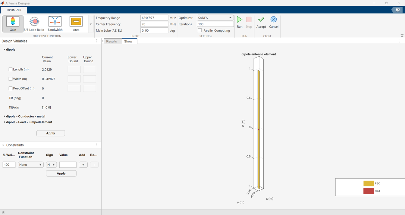
Use options from the OBJECTIVE FUNCTION menu to choose the main goal of antenna optimization.
Use the Design Variables panel to select variables and specify their bounds. The variables are then changed by the optimizer depending on their lower and upper bounds.
Use the Geometric Constraints panel to specify coefficient matrix corresponding to linear constraint equations of design variables, and nonlinear constraints.
Use constraint functions from the Analysis Constraints panel to restrict a desired analysis function value for the antenna. You can add multiple constraint functions along with their weightage.
Use the Optimizer menu to choose between
SADEA,Surrogate Opt, orTR-SADEAoptimizers.Note
To use Parallel Computing for
SADEAandTR-SADEAoptimizer, you need a Parallel Computing Toolbox license.
To use the Surrogate optimizer, you need a Global Optimization Toolbox license.
After adding the required values, click Run to start the optimization.
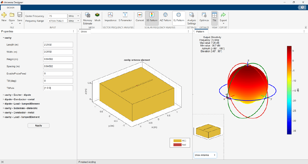
Use the Antenna Designer app to plot the radiation pattern of a cavity-backed dipole antenna.
Open the app and click New to show the default dipole antenna.
From the BACKING STRUCTURE GALLERY, click Rectangular Cavity to create a cavity-backed dipole antenna.
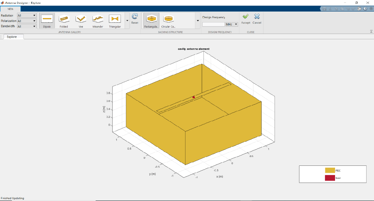
Click Accept.
In SCALAR FREQUENCY ANALYSIS, click 3D Pattern to calculate the radiation pattern of the cavity-backed dipole. The default frequency used is 75 MHz. Click Tile to view both the antenna and the radiation pattern.
Use the Antenna Designer app to plot the radiation pattern of a patch microstrip antenna with a dielectric substrate.
Open the app and click New. In the ANTENNA GALLERY section, under PATCH FAMILY, click Microstrip. Click Accept.
On the Antenna Properties tab, change the ground plane length and width to 0.120 m. Click Apply to see the changes.
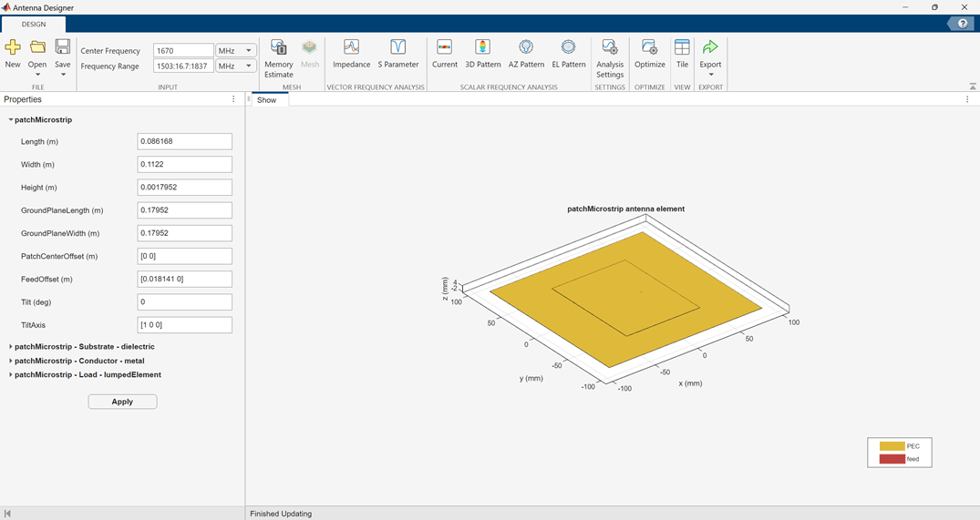
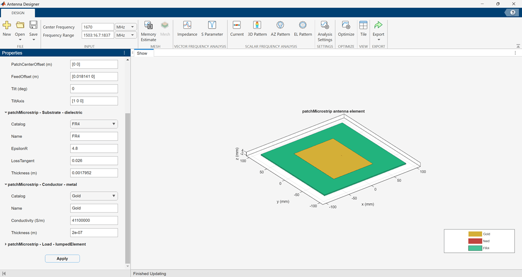
Add an FR4 dielectric as a substrate to the microstrip patch antenna. To add the dielectric, open the Substrate section and select required dielectric from the Dielectric Catalog drop-down. Set the substrate Name to FR4, EpsilonR to 4.8000, and Loss Tangent to 0.0260. Also add Gold metal as a conductor to the microstrip patch antenna. To add the metal, open the Conductor section and select required metal from the Metal Catalog drop-down. You can also use custom dielectric or metal materials by setting the fields: Name, EpsilonR, Loss Tangent, Conductivity and Thickness. Click Apply to see the antenna.
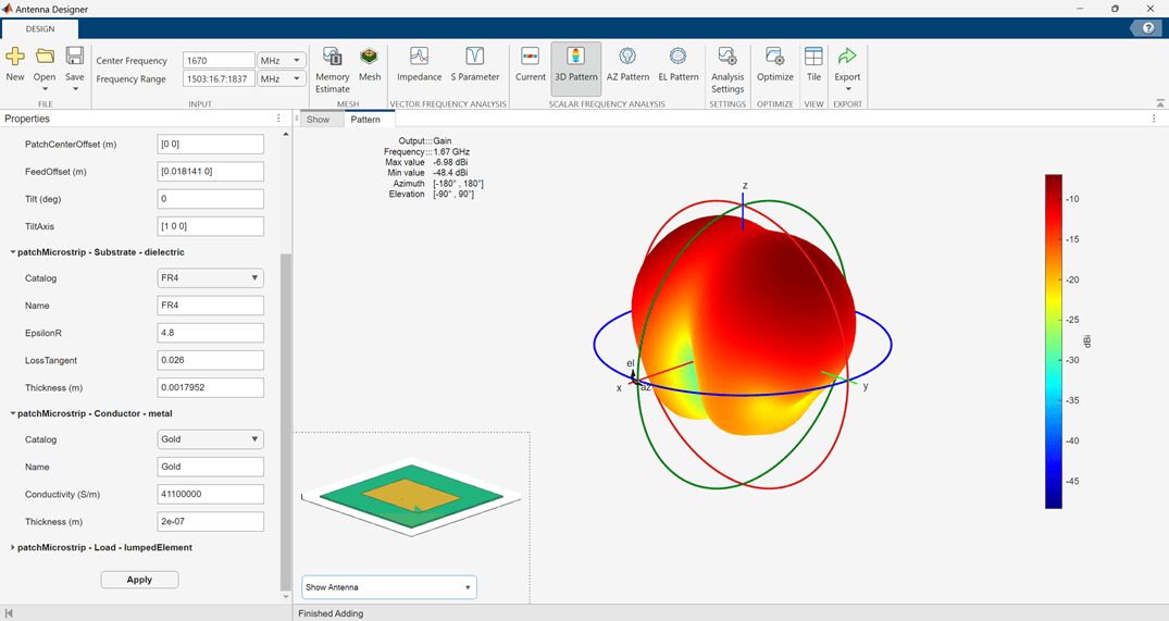
Click 3D Pattern to plot the radiation pattern of the antenna at the default frequency of 1.67 GHz.
Create and export a discone antenna using Antenna Designer app.
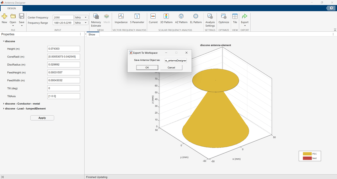
The exported antenna is visible in the MATLAB workspace in the form of a MAT file.
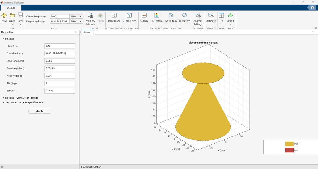
Change the parameters of the antenna to the below given values at the MATLAB command line and save the MAT file again to a known folder.
Rd = 55e-3;              % Radius of disc
Rc1 = 72.1e-3;           % Broad Radius of cone
Rc2 = 1.875e-3;          % Narrow Radius of cone
Hc = 160e-3;             % Vertical height of cone
Fw = 1e-3;               % Feed Width
S = 1.75e-3;             % Spacing between cone and disc
Open the updated MAT file of the discone antenna using the open button.
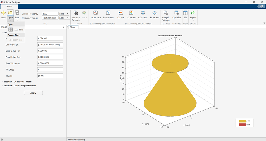
The app overwrites the previous discone antenna design and open the updated discone antenna.
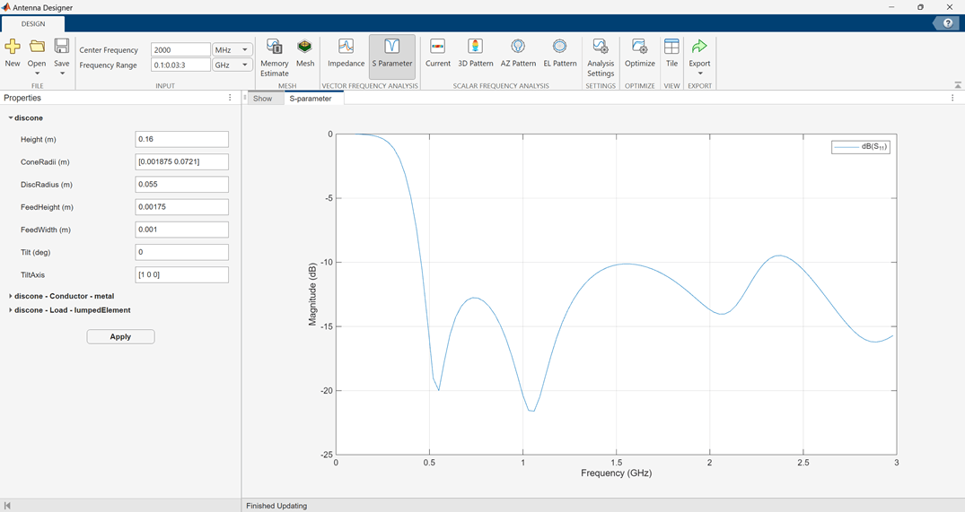
Calculate the S-parameter of the antenna at the specified frequency range.
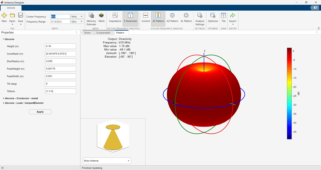
Plot the radiation pattern of the antenna at the specified frequency.
Minimize the occupied area of a dipole antenna such that gain of the antenna is greater than 4 dBi.
Open Antenna Designer app and accept the default dipole antenna.
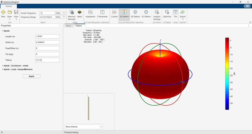
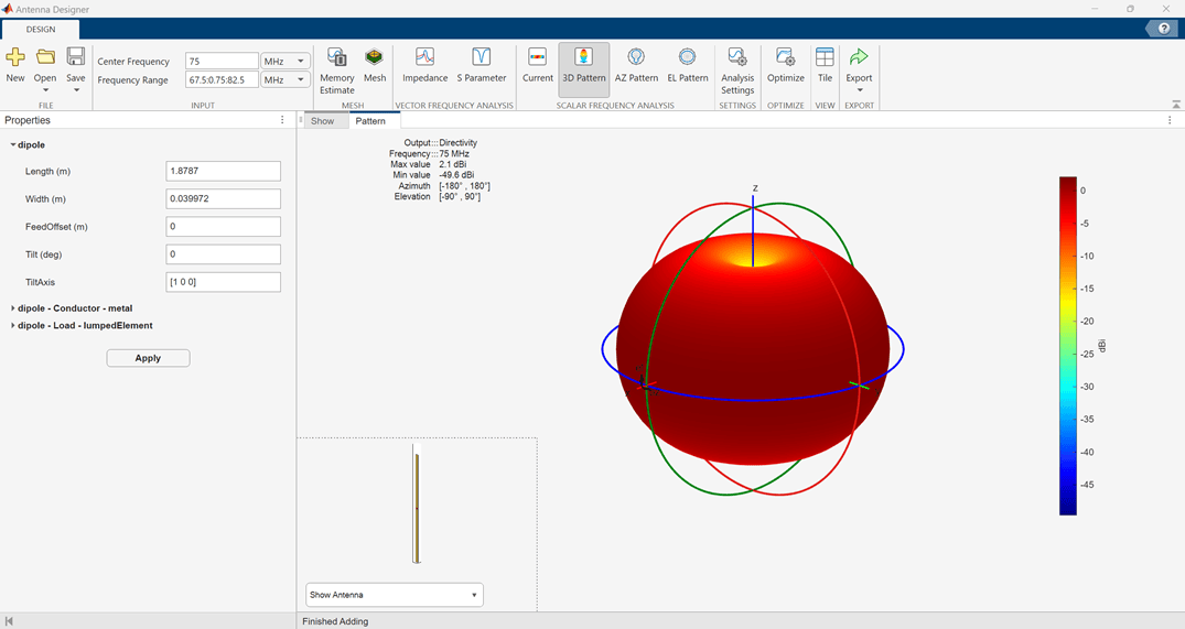
Analyze the pattern of the antenna. Notice that the Max value for directivity in the plot is 2.1 dBi.
Optimize Dipole Antenna
Click on Optimize to open the Optimizer canvas of the Antenna Designer app.
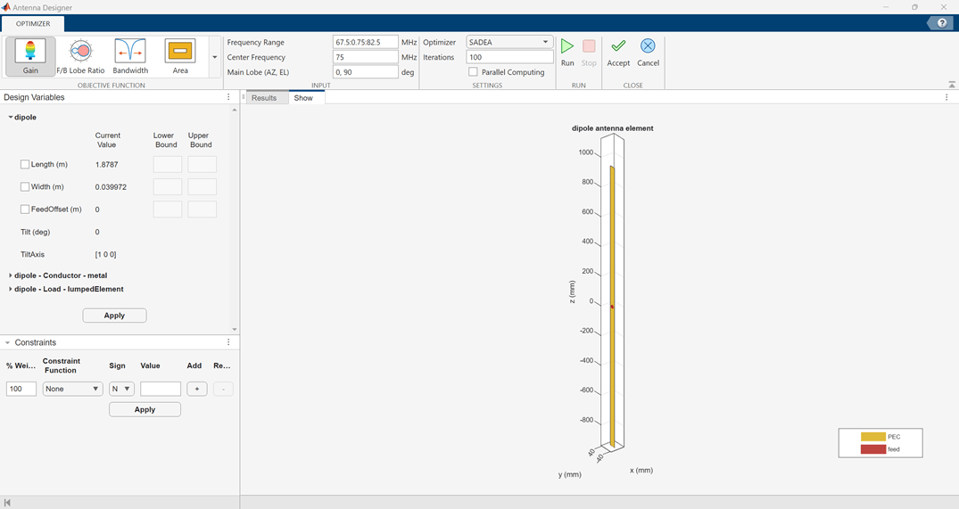
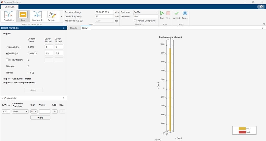
From the OBJECTIVE FUNCTION drop down choose, Minimize Area. Enter the bounds for the length and the width of the antenna in the Design Variables tab. Click Apply.
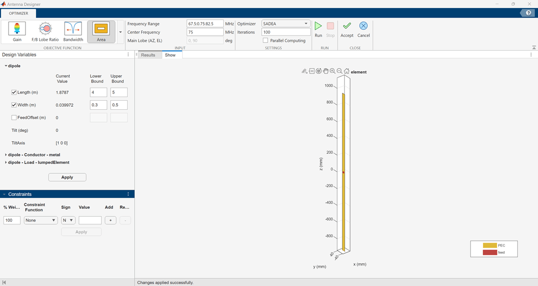
Enter the constraints in the Constraints tab. Click Apply.
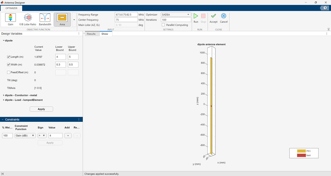
Set the number of iterations to 50. Click Run.
First the optimizer builds the model.
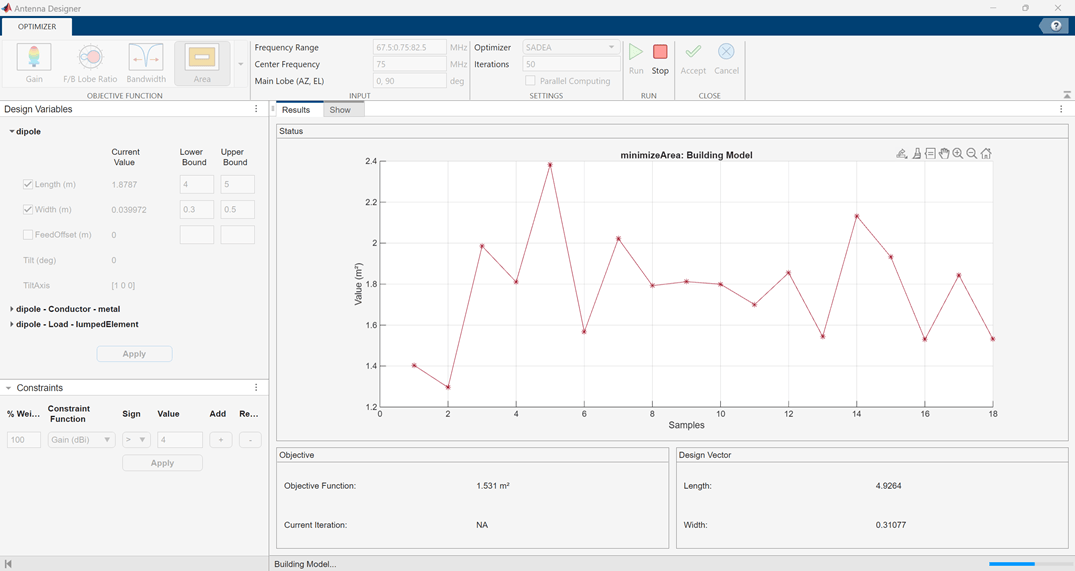
Then starts the optimization based on the objective function and the constraints.
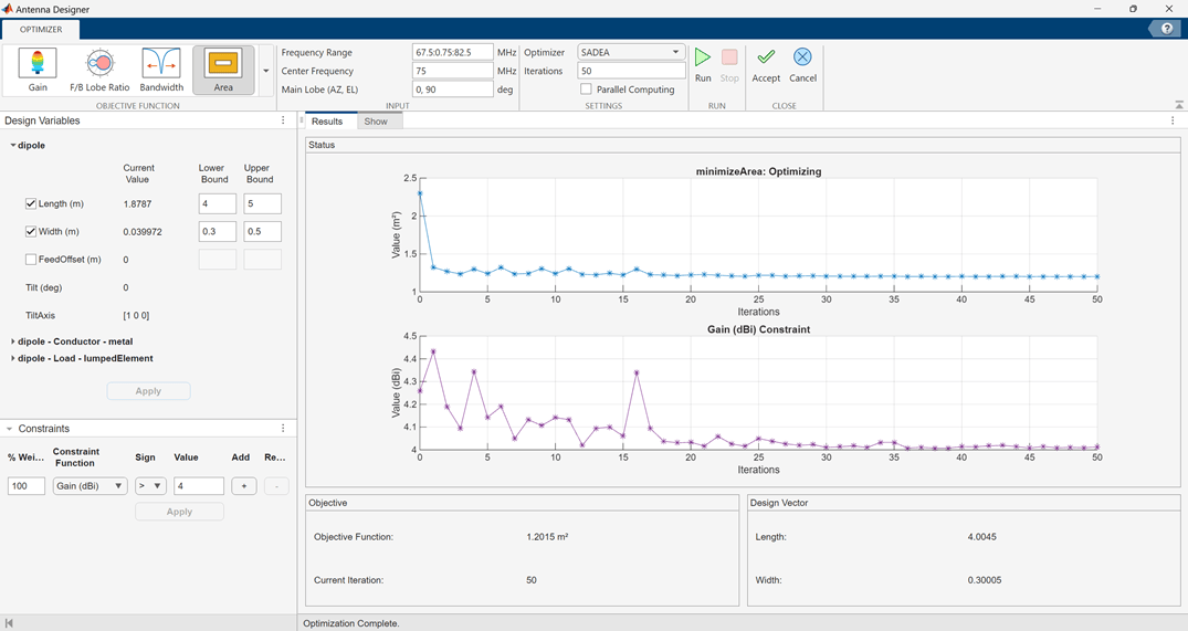
Click Accept.
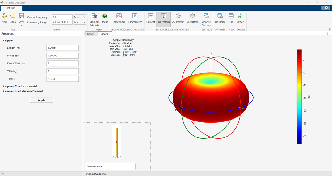
Analyze the antenna again for the 3D pattern. See that the Max value of the directivity is now 4.01 dBi.
Minimize the occupied area of a dipole antenna such that gain of the antenna is greater than 4 dBi.
Open Antenna Designer app and accept the default dipole antenna.
Analyze the pattern of the antenna. Notice that the Max value for directivity in the plot is 2.1 dBi.
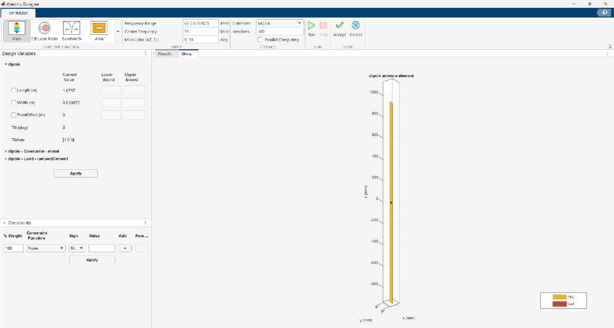
Optimize Dipole Antenna
Click on Optimize to open the Optimizer canvas of the Antenna Designer app.
From the OBJECTIVE FUNCTION drop down choose, Minimize Area. Enter the bounds for the length and the width of the antenna in the Design Variables tab. Click Apply.
Enter the constraints in the Constraints tab. Click Apply.
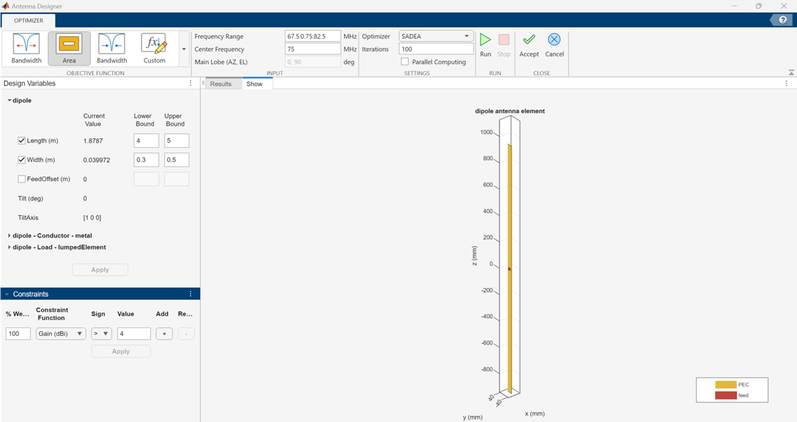
Change the Optimizer from SADEA to Surrogate Opt. The number iterations is always 200 and Parallel Computing is grayed out. Click Run.
The optimization starts based on the objective function and the constraints.
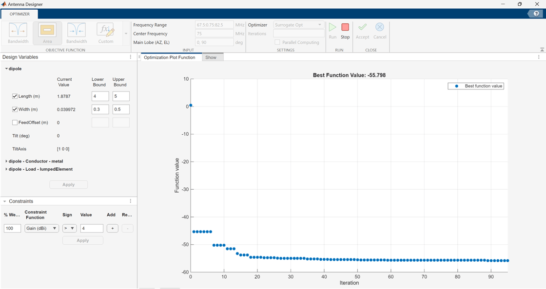
Click Accept.
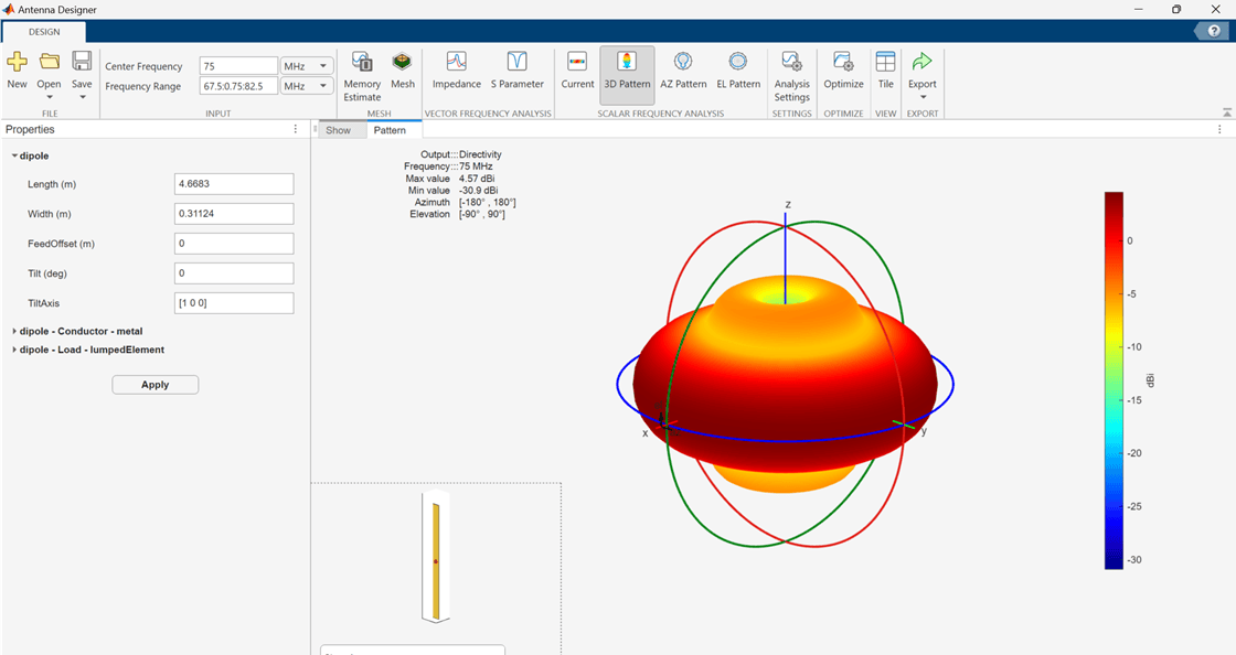
Analyze the antenna again for the 3D pattern. See that the Max value of the directivity is now 4.57 dBi.
Related Examples
Programmatic Use
Version History
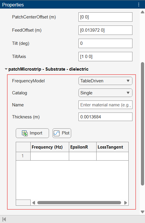
Introduced in R2017aThe Antenna Designer app now lets you choose a dispersion model to include the effect of frequency variation on the dielectric properties of the material. The supported dispersion models are constant, Djordjevic-Sarkar, the mean of Djordjevic-Sarkar, and table driven. To specify a dispersion model, use the new FrequencyModel parameter in the property panel with one of these values:
Constant— Dielectric material properties remain constant throughout the frequency range.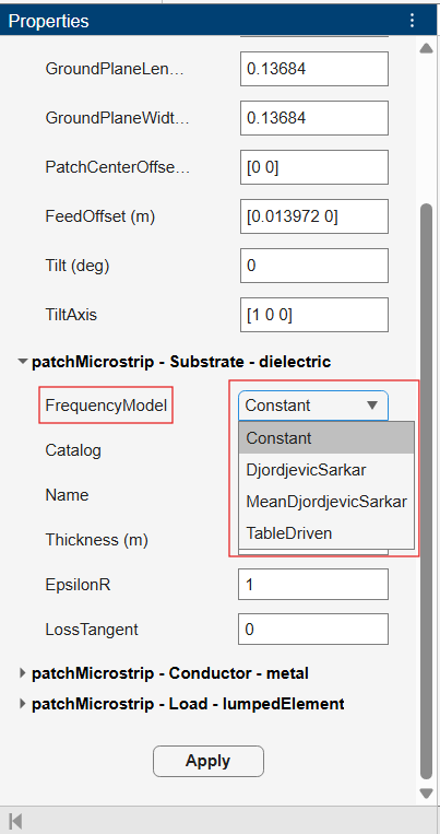
DjordjevicSarkar— Dielectric material properties follow Djordjevic-Sarkar model for the specified frequency. To specify a frequency for the dielectric material, use the new Frequency parameter in the property panel.
MeanDjordjevicSarkar— Calculates and uses the mean of Djordjevic-Sarker model over the frequency range for the dielectric material properties. To specify a frequency for the dielectric material, use the new Frequency parameter in the property panel.
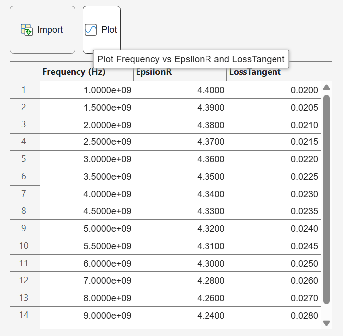
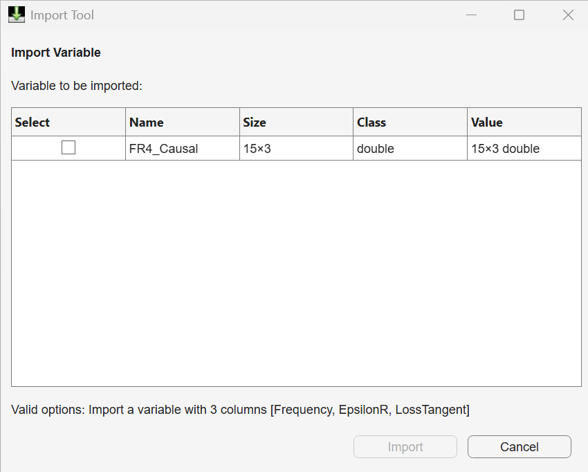
TableDriven— Uses a rational fit on the data provided for dielectric material properties.You can manually fill the frequency, relative permittivity, and loss tangent data to the table. To import the data from a workspace variable, click Import.
Select a variable from the list, and click Import.
To plot the relative permittivity and loss tangent of the material as a function of the frequency, click Plot.