Digital DATCOM Data
Digital DATCOM Data Overview
To import United States Air Force (USAF) Digital DATCOM files into the MATLAB® environment, use the datcomimport function. For more
information, see the datcomimport function reference page. This
topic explains how to import data from a USAF Digital DATCOM file using the Import from USAF Digital DATCOM Files example.
USAF Digital DATCOM File
Aerospace Toolbox provides astdatcom.in, a sample input file for USAF Digital DATCOM for
a wing-body-horizontal tail-vertical tail configuration running over five alphas, two Mach
numbers, and two altitudes. It calculates static and dynamic derivatives.
 $FLTCON NMACH=2.0,MACH(1)=0.1,0.2$
 $FLTCON NALT=2.0,ALT(1)=5000.0,8000.0$
 $FLTCON NALPHA=5.,ALSCHD(1)=-2.0,0.0,2.0,
  ALSCHD(4)=4.0,8.0,LOOP=2.0$
 $OPTINS SREF=225.8,CBARR=5.75,BLREF=41.15$
 $SYNTHS XCG=7.08,ZCG=0.0,XW=6.1,ZW=-1.4,ALIW=1.1,XH=20.2,
   ZH=0.4,ALIH=0.0,XV=21.3,ZV=0.0,VERTUP=.TRUE.$
 $BODY NX=10.0,
   X(1)=-4.9,0.0,3.0,6.1,9.1,13.3,20.2,23.5,25.9,
   R(1)=0.0,1.0,1.75,2.6,2.6,2.6,2.0,1.0,0.0$
 $WGPLNF CHRDTP=4.0,SSPNE=18.7,SSPN=20.6,CHRDR=7.2,SAVSI=0.0,CHSTAT=0.25,
   TWISTA=-1.1,SSPNDD=0.0,DHDADI=3.0,DHDADO=3.0,TYPE=1.0$
NACA-W-6-64A412
 $HTPLNF CHRDTP=2.3,SSPNE=5.7,SSPN=6.625,CHRDR=0.25,SAVSI=11.0,
   CHSTAT=1.0,TWISTA=0.0,TYPE=1.0$
NACA-H-4-0012
 $VTPLNF CHRDTP=2.7,SSPNE=5.0,SSPN=5.2,CHRDR=5.3,SAVSI=31.3,
   CHSTAT=0.25,TWISTA=0.0,TYPE=1.0$
NACA-V-4-0012
CASEID SKYHOGG BODY-WING-HORIZONTAL TAIL-VERTICAL TAIL CONFIG
DAMP
NEXT CASE
To view the output file generated by USAF Digital DATCOM for the same
wing-body-horizontal tail-vertical tail configuration running over five alphas, two Mach
numbers, and two altitudes, type
astdatcom.out in the MATLAB Command Window.
Data from DATCOM Files
To import Digital DATCOM data into the MATLAB environment, use the datcomimport function.
alldata = datcomimport('astdatcom.out', true, 0);Imported DATCOM Data
The datcomimport function creates a cell array of structures
containing the data from the Digital DATCOM output file.
data = alldata{1}
data =
 struct with fields:

        case: 'SKYHOGG BODY-WING-HORIZONTAL TAIL-VERTICAL TAIL CONFIG'
        mach: [0.1000 0.2000]
         alt: [5000 8000]
       alpha: [-2 0 2 4 8]
       nmach: 2
        nalt: 2
      nalpha: 5
       rnnub: []
      hypers: 0
        loop: 2
        sref: 225.8000
        cbar: 5.7500
       blref: 41.1500
         dim: 'ft'
       deriv: 'deg'
      stmach: 0.6000
      tsmach: 1.4000
        save: 0
       stype: []
        trim: 0
        damp: 1
       build: 1
        part: 0
     highsym: 0
     highasy: 0
     highcon: 0
        tjet: 0
      hypeff: 0
          lb: 0
         pwr: 0
        grnd: 0
       wsspn: 18.7000
       hsspn: 5.7000
      ndelta: 0
       delta: []
      deltal: []
      deltar: []
         ngh: 0
      grndht: []
      config: [1x1 struct]
          cd: [5x2x2 double]
          cl: [5x2x2 double]
          cm: [5x2x2 double]
          cn: [5x2x2 double]
          ca: [5x2x2 double]
         xcp: [5x2x2 double]
         cla: [5x2x2 double]
         cma: [5x2x2 double]
         cyb: [5x2x2 double]
         cnb: [5x2x2 double]
         clb: [5x2x2 double]
       qqinf: [5x2x2 double]
         eps: [5x2x2 double]
    depsdalp: [5x2x2 double]
         clq: [5x2x2 double]
         cmq: [5x2x2 double]
        clad: [5x2x2 double]
        cmad: [5x2x2 double]
         clp: [5x2x2 double]
         cyp: [5x2x2 double]
         cnp: [5x2x2 double]
         cnr: [5x2x2 double]
         clr: [5x2x2 double]
Missing DATCOM Data
By default, the function sets missing data points to 99999. It sets data points to NaN when no DATCOM methods exist or when the method is not applicable.
It can be seen in the Digital DATCOM output file and examining the imported data that , , , and have data only in the first alpha value. Here are the imported data values.
data.cyb
ans(:,:,1) =

  1.0e+004 *

   -0.0000   -0.0000
    9.9999    9.9999
    9.9999    9.9999
    9.9999    9.9999
    9.9999    9.9999


ans(:,:,2) =

  1.0e+004 *

   -0.0000   -0.0000
    9.9999    9.9999
    9.9999    9.9999
    9.9999    9.9999
    9.9999    9.9999

data.cnb
ans(:,:,1) =

  1.0e+004 *

    0.0000    0.0000
    9.9999    9.9999
    9.9999    9.9999
    9.9999    9.9999
    9.9999    9.9999


ans(:,:,2) =

  1.0e+004 *

    0.0000    0.0000
    9.9999    9.9999
    9.9999    9.9999
    9.9999    9.9999
    9.9999    9.9999

data.clq
ans(:,:,1) =

  1.0e+004 *

    0.0000    0.0000
    9.9999    9.9999
    9.9999    9.9999
    9.9999    9.9999
    9.9999    9.9999


ans(:,:,2) =

  1.0e+004 *

    0.0000    0.0000
    9.9999    9.9999
    9.9999    9.9999
    9.9999    9.9999
    9.9999    9.9999

data.cmq
ans(:,:,1) =

  1.0e+004 *

   -0.0000   -0.0000
    9.9999    9.9999
    9.9999    9.9999
    9.9999    9.9999
    9.9999    9.9999


ans(:,:,2) =

  1.0e+004 *

   -0.0000   -0.0000
    9.9999    9.9999
    9.9999    9.9999
    9.9999    9.9999
    9.9999    9.9999
The missing data points are filled with the values for the first alpha, since these data points are meant to be used for all alpha values.
aerotab = {'cyb' 'cnb' 'clq' 'cmq'};

for k = 1:length(aerotab)
    for m = 1:data.nmach
        for h = 1:data.nalt
            data.(aerotab{k})(:,m,h) = data.(aerotab{k})(1,m,h);
        end
    end
end
The updated imported data values are:
data.cyb
ans(:,:,1) =

   -0.0035   -0.0035
   -0.0035   -0.0035
   -0.0035   -0.0035
   -0.0035   -0.0035
   -0.0035   -0.0035


ans(:,:,2) =

   -0.0035   -0.0035
   -0.0035   -0.0035
   -0.0035   -0.0035
   -0.0035   -0.0035
   -0.0035   -0.0035

data.cnb
ans(:,:,1) =

  1.0e-003 *

    0.9142    0.8781
    0.9142    0.8781
    0.9142    0.8781
    0.9142    0.8781
    0.9142    0.8781


ans(:,:,2) =

  1.0e-003 *

    0.9190    0.8829
    0.9190    0.8829
    0.9190    0.8829
    0.9190    0.8829
    0.9190    0.8829

data.clq
ans(:,:,1) =

    0.0974    0.0984
    0.0974    0.0984
    0.0974    0.0984
    0.0974    0.0984
    0.0974    0.0984


ans(:,:,2) =

    0.0974    0.0984
    0.0974    0.0984
    0.0974    0.0984
    0.0974    0.0984
    0.0974    0.0984

data.cmq
ans(:,:,1) =

   -0.0892   -0.0899
   -0.0892   -0.0899
   -0.0892   -0.0899
   -0.0892   -0.0899
   -0.0892   -0.0899


ans(:,:,2) =

   -0.0892   -0.0899
   -0.0892   -0.0899
   -0.0892   -0.0899
   -0.0892   -0.0899
   -0.0892   -0.0899
Aerodynamic Coefficients
You can now plot the aerodynamic coefficients:
Plotting Lift Curve Moments
h1 = figure;
figtitle = {'Lift Curve' ''};
for k=1:2
    subplot(2,1,k)
    plot(data.alpha,permute(data.cl(:,k,:),[1 3 2]))
    grid
    ylabel(['Lift Coefficient (Mach =' num2str(data.mach(k)) ')'])
    title(figtitle{k});
end
xlabel('Angle of Attack (deg)')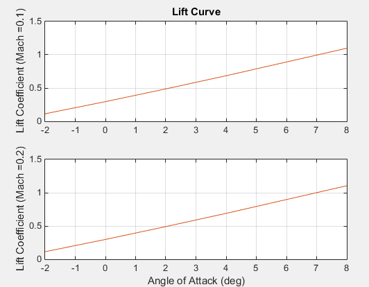
Plotting Drag Polar Moments
h2 = figure;
figtitle = {'Drag Polar' ''};
for k=1:2
    subplot(2,1,k)
    plot(permute(data.cd(:,k,:),[1 3 2]),permute(data.cl(:,k,:),[1 3 2]))
    grid
    ylabel(['Lift Coefficient (Mach =' num2str(data.mach(k)) ')'])
    title(figtitle{k})
end
xlabel('Drag Coefficient')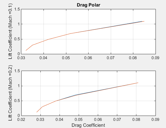
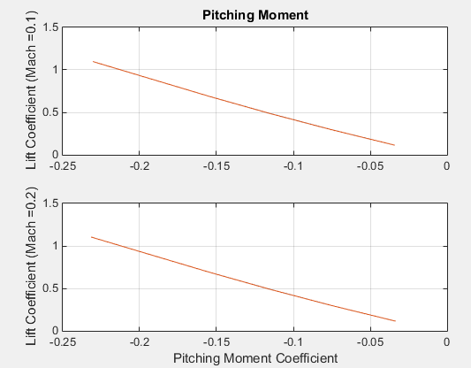
Plotting Pitching Moments
h3 = figure;
figtitle = {'Pitching Moment' ''};
for k=1:2
    subplot(2,1,k)
    plot(permute(data.cm(:,k,:),[1 3 2]),permute(data.cl(:,k,:),[1 3 2]))
    grid
    ylabel(['Lift Coefficient (Mach =' num2str(data.mach(k)) ')'])
    title(figtitle{k})
end
xlabel('Pitching Moment Coefficient')