Train and Evaluate Neural Networks for 5G MIMO Channel Estimation

R2026b

Since R2026b

This example shows how to train, evaluate, and compare neural network architectures for 5G NR MIMO channel estimation using MATLAB® and 5G Toolbox®. Deploying a neural network for channel estimation involves many design choices: architecture, input representation, and side information to condition the network. This example showcases a modular workflow that lets you swap architecture or input representation and measure the impact on channel estimation and throughput performance.

The example explores the following design choices:

• Architecture: Define how the network processes the resource grid: ViT (self-attention), CENet (MLP-Mixer), and ResDenoiser (deep residual CNN).

• Input representation: Define the channel estimate that the network receives as its starting point: practical (output of nrChannelEstimate), ls-interp (LS estimates linearly interpolated across the resource grid), and ls-sparse (LS estimates at pilot resource elements (REs) only, with a binary mask indicating pilot positions).

• Antenna-layer processing: Define how antenna-layer pairs are processed: each (Rx antenna, layer) pair is processed independently, making the network antenna-configuration agnostic. With SVD precoding, the effective channel has orthogonal columns across layers, so each (Rx antenna, layer) pair is independent and processed separately, making the network antenna-configuration agnostic. The network does not require SVD specifically. It processes each column of the effective channel independently and learns to map imperfect inputs to the ideal channel response, so it can tolerate precoder mismatches (for example, from channel aging).

• Feature-wise linear modulation (FiLM) conditioning: Condition the network on SNR to adapt denoising and interpolation strength.

• Precoding resource block group (PRG) tiling: Tile the resource grid to enable bandwidth-agnostic inference by processing one 4-RB PRG at a time.

For information on channel estimation using a simple CNN (SISO, single architecture), see Train Low Complexity CNN for 5G SISO Channel Estimation.

For a step-by-step explanation of MIMO data generation and input preprocessing used in this example, see Generate Data for AI-Based 5G MIMO Channel Estimation.

System Configuration

Configure a 5G NR downlink with 2x2 MIMO. The hDeepLearningChanEstSimParameters helper function configures system and channel parameters. Some of these parameters directly affect channel estimation performance. In particular, channel estimation relies on DM-RS pilot symbols inserted into the OFDM grid, and the DM-RS configuration controls pilot density in both time and frequency:

• DMRSAdditionalPosition=1 places pilots in 2 OFDM symbols per slot, providing two time-domain snapshots for interpolation.

• ConfigType=1 with CombFactor=2 provides 6 pilot subcarriers per RB, resulting in approximately 7% RE overhead.

At moderate Doppler (up to approximately 100 Hz with TDL-C, 300 ns delay spread), two time-domain pilot symbols are sufficient for the practical estimator to reach 100% throughput at high SNR. At higher Doppler or longer delay spreads, the practical estimator degrades, leaving more room for neural networks to improve.

hDeepLearningChanEstSimParameters returns default parameters. To customize, pass name-value arguments such as NSizeGrid, NTxAnts, NRxAnts, SubcarrierSpacing, or DMRSAdditionalPosition.

simParameters = hDeepLearningChanEstSimParameters();
% simParameters = hDeepLearningChanEstSimParameters(DMRSAdditionalPosition=3, NTxAnts=4);
disp("Carrier: " + simParameters.Carrier.NSizeGrid + " RBs, " ...
    + simParameters.Carrier.SubcarrierSpacing + " kHz SCS")

Carrier: 52 RBs, 15 kHz SCS

disp("Antenna: " + simParameters.NTxAnts + " Tx x " ...
    + simParameters.NRxAnts + " Rx, " ...
    + simParameters.PDSCH.NumLayers + " layers")

Antenna: 2 Tx x 2 Rx, 2 layers

disp("DM-RS: AddPos=" + simParameters.PDSCH.DMRS.DMRSAdditionalPosition ...
    + ", ConfigType=" + simParameters.PDSCH.DMRS.DMRSConfigurationType)

DM-RS: AddPos=1, ConfigType=1

disp("Modulation: " + string(simParameters.PDSCH.Modulation))

Modulation: 16QAM

carrier = simParameters.Carrier;
pdsch = simParameters.PDSCH;
Nsc = carrier.NSizeGrid * 12;
Nsym = carrier.SymbolsPerSlot;

Neural Network Input Representations

The input to the neural network is a design choice. The received resource grid contains pilot symbols (DM-RS) at known positions. A least-squares (LS) estimate at those positions gives the raw channel observation. You can feed the network this raw observation directly, or first interpolate and smooth it to fill the entire grid. Each choice trades off noise reduction against estimation bias:

• LS-Sparse: LS estimates at pilot RE positions only, zeros elsewhere. A binary mask channel (1 at pilot REs, 0 elsewhere) tells the network which positions contain actual measurements. The network learns both interpolation and denoising from the pilot observations. LS estimation is inherently unbiased at pilot positions, so the network starts from raw but accurate observations.

• LS-Interp: LS estimates extended to all REs via linear interpolation in frequency and time. The network receives a full grid, so it only needs to denoise. However, linear interpolation does not suppress noise. It only fills gaps between pilots. It also introduces bias when the channel does not change linearly between pilot positions.

• Practical: Output of nrChannelEstimate, which applies CIR-domain denoising, spline frequency interpolation, and linear time interpolation. This produces a dense estimate with lower noise variance at low SNR, but smoothing and interpolation remove channel detail, creating a bias floor at high SNR.

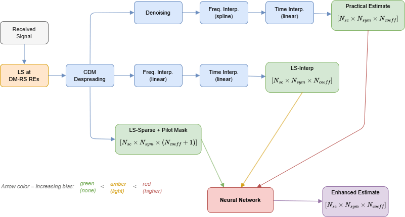
The hGenerate5GChannelEstimationData helper function simulates the channel once and returns all representations of the same realization, enabling fair side-by-side comparison. Visualize the channel estimation magnitude for one PRG (48 subcarriers x 14 OFDM symbols, first antenna-layer pair) at 20 dB SNR. Each panel shows the same channel realization estimated with a different method, from sparse pilot observations (left) to the perfect channel (right). This visualization is for illustration only and is not used to train the network.

sampleData = hGenerate5GChannelEstimationData(1, SNRRange=[20 20], DopplerRange=[100 100], ...
    DelaySpreadRange=[300 300], SeedRange=[1 1], SimParameters=simParameters);
plotChannelRepresentations(sampleData);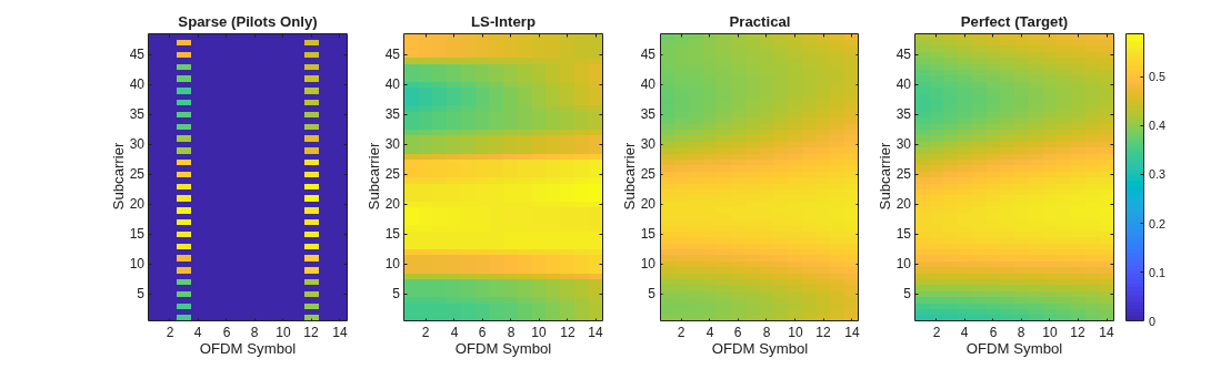

Generate and Prepare Training Data

Generate channel realizations (each realization is one independent slot with SNR, Doppler, and delay spread drawn uniformly from the specified ranges, and independent channel fading) with all input representations and prepare neural network ready training arrays. For a step-by-step explanation of data generation and input preparation (PRG tiling, real/imaginary interleaving, RMS normalization, side information), see Train Low Complexity CNN for 5G SISO Channel Estimation.

For faster interactive execution, set numRealizations to 256. For more accurate training, set numRealizations to 4096.

dopplerRange = [5 400];
delaySpreadRange = [30 1000];
delayProfiles = {"TDL-A", "TDL-C", "TDL-D"}; % 2 NLOS + 1 LOS
snrRange = [-5 25];
prgSizeRBs = 4;
numRealizations = 256; %4096;

if ~exist("trainX", "var")
    [pracData,interpData,sparseData,trainX,valX,nCh] = prepareData(numRealizations,snrRange,dopplerRange,delaySpreadRange,delayProfiles,simParameters,prgSizeRBs);
end

Realizations: 256

disp("Training samples: " + size(trainX, 4) + " (" ...
    + size(trainX,1) + "x" + size(trainX,2) + "x" + size(trainX,3) + ")")

Training samples: 11960 (48x14x2)

disp("Validation samples: " + size(valX, 4))

Validation samples: 1352

Build Neural Network

This example provides three architectures. Select one to build and train:

• ViT: Vision Transformer with patch embedding and multi-head self-attention. Captures long-range correlations across frequency and time through global interactions between resource grid positions. Computationally intensive but well suited to modeling global channel structure. See hBuildChanEstViT.

• CENet: MLP-Mixer with depth-wise separable convolutions and token mixing. Combines local feature extraction with spatial mixing across the resource grid. Lightweight but provides a more limited receptive field than ViT. See hBuildChanEstCENet.

• ResDenoiser: Deep residual CNN that learns to predict and subtract channel estimation errors. Efficient for denoising and refining local channel structure. Strong for denoising but less effective for sparse reconstruction than ViT. See hBuildChanEstResDenoiser.

Select the architecture and input representation:

architectureName = "ViT";
inputType = "ls-sparse";

Build the selected network.

NscPRG = prgSizeRBs * 12;
useMask = inputType == "ls-sparse";
switch inputType
    case "ls-sparse"
        selectedData = sparseData;
    case "ls-interp"
        selectedData = interpData;
    case "practical"
        selectedData = pracData;
end
switch architectureName
    case "ViT"
        net = hBuildChanEstViT(NscPRG, Nsym, 64, NumBlocks=4, ...
            SNRConditioning=true, InOutChannels=nCh, MaskInput=useMask);
    case "CENet"
        net = hBuildChanEstCENet(NscPRG, Nsym, DropoutRate=0.1, ...
            TokenMixHidden=256, SNRConditioning=true, InOutChannels=nCh, MaskInput=useMask);
    case "ResDenoiser"
        net = hBuildChanEstResDenoiser(NscPRG, Nsym, NumFilters=64, ...
            SNRConditioning=true, InOutChannels=nCh, MaskInput=useMask);
end
net = initialize(net);

Display the network summary to verify the architecture size and input dimensions. Deep Learning Toolbox® uses image input layers for any 2D spatial data. Here, the 48x14 "image" is the resource grid (subcarriers x OFDM symbols).

summary(net)

   Initialized: true

   Number of learnables: 152.8k

   Inputs:
      1   'resource_grid'   48×14×2 images
      2   'mask_input'      48×14×1 images
      3   'snr_input'       1 features

FiLM Conditioning: SNR Adaptation

The optimal behavior of a channel estimator depends on operating conditions. At low SNR values, the network must denoise aggressively, smoothing out noise at the cost of rapid channel variations in frequency or time. At high SNR values, noise is minimal and the network must preserve these variations rather than oversmoothing them.

Rather than training separate networks for each SNR regime, all three architectures use FiLM [1] conditioning. By providing the estimated SNR value to the network as side information, FiLM allows a single network to adapt its denoising strength to the current operating point. Internally, the SNR scalar passes through two fully connected layers to produce a bias vector that shifts the internal feature maps of the network.

SNR Conditioning

The estimated per-slot SNR is normalized to the range 0 to 1:

$$

$$c_{\text{SNR}}=\frac{{\text{SNR}}_{\text{dB}}-{\text{SNR}}_{\text{min}}}{{\text{SNR}}_{\text{max}}-{\text{SNR}}_{\text{min}}}$$

$$

All pretrained models in this example use SNRConditioning=true with SNR_min = –10 dB and SNR_max = 30 dB. At inference, the SNR is estimated from the received signal power and noise variance.

Train Network

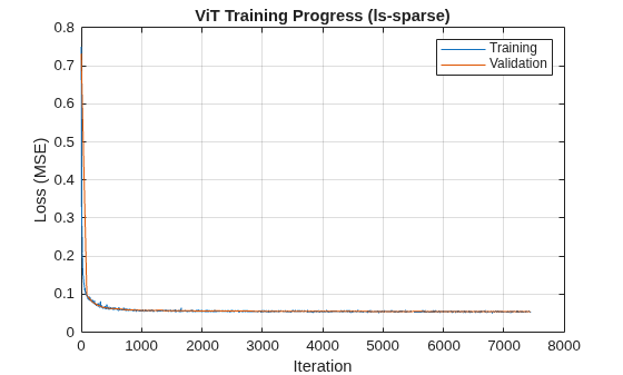
Train the selected network using the Adam optimizer with a piecewise learning rate schedule. The network minimizes mean-squared error between its output and the perfect channel response. Training uses the best-validation-loss checkpoint to prevent overfitting. Set trainNow to false to load a pretrained model. To reproduce all shipped pretrained models and evaluation results from scratch, use hReproduceAIMIMOChannelEstimationResults.

trainNow = false;

Map architecture and input type to pretrained model filename.

trainX = selectedData.trainX;
trainT = selectedData.trainT;
valX = selectedData.valX;
valT = selectedData.valT;
trainSNR = selectedData.trainSNR;
valSNR = selectedData.valSNR;
dataFolder = "mimoceData";
if trainNow
    nTrain = size(trainX, 4);
    nVal = size(valX, 4);
    if useMask
        trainCells = cell(nTrain, 4);
        for i = 1:nTrain
            trainCells{i,1} = trainX(:,:,:,i);
            trainCells{i,2} = selectedData.trainMask(:,:,:,i);
            trainCells{i,3} = single(trainSNR(i));
            trainCells{i,4} = trainT(:,:,:,i);
        end
        valCells = cell(nVal, 4);
        for i = 1:nVal
            valCells{i,1} = valX(:,:,:,i);
            valCells{i,2} = selectedData.valMask(:,:,:,i);
            valCells{i,3} = single(valSNR(i));
            valCells{i,4} = valT(:,:,:,i);
        end
    else
        trainCells = cell(nTrain, 3);
        for i = 1:nTrain
            trainCells{i,1} = trainX(:,:,:,i);
            trainCells{i,2} = single(trainSNR(i));
            trainCells{i,3} = trainT(:,:,:,i);
        end
        valCells = cell(nVal, 3);
        for i = 1:nVal
            valCells{i,1} = valX(:,:,:,i);
            valCells{i,2} = single(valSNR(i));
            valCells{i,3} = valT(:,:,:,i);
        end
    end
    trainDS = arrayDatastore(trainCells, OutputType="same", IterationDimension=1);
    valDS = arrayDatastore(valCells, OutputType="same", IterationDimension=1);
    batchSize = 256;
    iterPerEpoch = floor(nTrain / batchSize);
    options = trainingOptions("adam", ...
        InitialLearnRate=1e-3, ...
        LearnRateSchedule="piecewise", ...
        LearnRateDropFactor=0.55, ...
        LearnRateDropPeriod=5, ...
        MaxEpochs=80, ...
        MiniBatchSize=batchSize, ...
        Shuffle="every-epoch", ...
        Verbose=false, ...
        Plots="training-progress", ...
        ValidationData=valDS, ...
        ValidationFrequency=max(1, iterPerEpoch), ...
        ValidationPatience=Inf, ...
        OutputNetwork="best-validation-loss", ...
        ExecutionEnvironment="auto");
    [trainedNet, trainingInfo] = trainnet(trainDS, net, "mean-squared-error", options);
    vLoss = trainingInfo.ValidationHistory.Loss;
    vLoss = vLoss(~isnan(vLoss));
    disp("Best validation loss: " + min(vLoss))

    networkMeta.InputType = inputType;
    networkMeta.PerAntennaLayer = true;
    networkMeta.SNRConditioning = true;
    networkMeta.SNRRange = snrRange;
    networkMeta.PRGSizeRBs = prgSizeRBs;
    networkMeta.DMRSSymbolIndices = selectedData.dmrsSymIdx;
    networkMeta.PilotMask = single(selectedData.pilotMask);

    archTag = lower(architectureName);
    inputTag = replace(inputType, "ls-sparse", "ls_sparse_mask");
    inputTag = replace(inputTag, "ls-interp", "ls_interp");
    addPos = simParameters.PDSCH.DMRS.DMRSAdditionalPosition;
    dop = round(mean(dopplerRange));
    timestamp = string(datetime("now", "Format", "yyyyMMdd'T'HHmm"));
    modelFile = fullfile(dataFolder, "trained_" + archTag + "_" + inputTag ...
        + "_addpos" + addPos + "_dop" + dop + "_" + timestamp + ".mat");
    save(modelFile, "trainedNet", "networkMeta", "trainingInfo");
    fprintf("Saved: %s\n", modelFile);
else
    modelFiles = dictionary( ...
        "ViT-practical", fullfile(dataFolder,"trained_vit_practical_addpos1.mat"), ...
        "ViT-ls-interp", fullfile(dataFolder,"trained_vit_ls_interp_addpos1.mat"), ...
        "ViT-ls-sparse", fullfile(dataFolder,"trained_vit_ls_sparse_mask_addpos1.mat"), ...
        "CENet-practical", fullfile(dataFolder,"trained_cenet_practical_addpos1.mat"), ...
        "CENet-ls-interp", fullfile(dataFolder,"trained_cenet_ls_interp_addpos1.mat"), ...
        "CENet-ls-sparse", fullfile(dataFolder,"trained_cenet_ls_sparse_mask_addpos1.mat"), ...
        "ResDenoiser-practical", fullfile(dataFolder,"trained_resden_practical_addpos1.mat"), ...
        "ResDenoiser-ls-interp", fullfile(dataFolder,"trained_resden_ls_interp_addpos1.mat"), ...
        "ResDenoiser-ls-sparse", fullfile(dataFolder,"trained_resden_ls_sparse_mask_addpos1.mat"));
    modelKey = architectureName + "-" + inputType;
    S = load(modelFiles(modelKey));
    trainedNet = S.trainedNet;
    networkMeta = S.networkMeta;
    trainingInfo = S.trainingInfo;
    vLoss = trainingInfo.ValidationHistory.Loss;
    vLoss = vLoss(~isnan(vLoss));
    disp("Loaded pretrained " + architectureName + " (" + inputType + ...
        "). Best validation loss: " + min(vLoss))
    figure
    plot(trainingInfo.TrainingHistory.Iteration, trainingInfo.TrainingHistory.Loss)
    hold on
    valIter = trainingInfo.ValidationHistory.Iteration;
    valLoss = trainingInfo.ValidationHistory.Loss;
    plot(valIter(~isnan(valLoss)), valLoss(~isnan(valLoss)))
    hold off
    xlabel("Iteration")
    ylabel("Loss (MSE)")
    title(architectureName + " Training Progress (" + inputType + ")")
    legend("Training", "Validation", Location="northeast")
    grid on
end

Loaded pretrained ViT (ls-sparse). Best validation loss: 0.054428

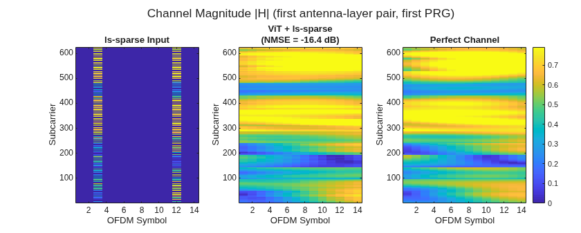
Run Inference on New Slot

Wrap the trained network in an hNNChannelEstimator System object for inference. The object handles PRG tiling, per-PRG RMS normalization, and SNR conditioning for the specified channel estimate.

estimator = hNNChannelEstimator(trainedNet, networkMeta);
slot = hGenerate5GChannelEstimationData(1, ...
    SNRRange=[10 10], DopplerRange=[300 300], ...
    DelaySpreadRange=[300 300], SeedRange=[42 42], ...
    SimParameters=simParameters);
nRx = simParameters.NRxAnts;
nLayers = simParameters.PDSCH.NumLayers;
perfectEst4D = reshape(slot.perfect, Nsc, Nsym, nRx, nLayers);

Select the input matching the trained model and run inference.

switch inputType
    case "practical"
        inputEst4D = reshape(slot.practical, Nsc, Nsym, nRx, nLayers);
        noiseVar = slot.noiseVarPractical;
    case "ls-interp"
        inputEst4D = reshape(slot.lsInterp, Nsc, Nsym, nRx, nLayers);
        noiseVar = slot.noiseVarLS;
    case "ls-sparse"
        inputEst4D = reshape(slot.lsSparse, Nsc, Nsym, nRx, nLayers);
        noiseVar = slot.noiseVarLS;
end
nnEst = estimator(inputEst4D, noiseVar);

Compute normalized mean squared error (NMSE) in dB for the input estimate and the NN output relative to the perfect channel.

nmseNN = 10*log10(mean(abs(nnEst(:) - perfectEst4D(:)).^2) / mean(abs(perfectEst4D(:)).^2));
plotInference(inputEst4D,inputType,nnEst,architectureName,nmseNN,perfectEst4D);

NMSE Evaluation: Architecture Comparison

Evaluate estimation quality using NMSE in dB, where $$H$$ is the perfect channel response and $$\underset{}{\overset{ˆ}{H}}$$ is the estimate:

$$

$$\text{NMSE}(\text{dB})=10{\log }_{10}\frac{\mathbb{E}[|\underset{}{\overset{ˆ}{H}}-H{|}^2]}{\mathbb{E}[|H{|}^2]}$$

$$

The hEvaluateChannelEstimationNMSE helper function runs a Monte Carlo simulation. For each SNR point, it generates independent channel realizations, transmits precoded PDSCH + DM-RS through the specified channel, and compares each estimator against the perfect OFDM channel response.

% Load trained networks (ls-sparse input)
vit = load("trained_vit_ls_sparse_mask_addpos1.mat","trainedNet","networkMeta");
cenet = load("trained_cenet_ls_sparse_mask_addpos1.mat","trainedNet","networkMeta");
resden = load("trained_resden_ls_sparse_mask_addpos1.mat","trainedNet","networkMeta");

% Build estimator objects
estVit = hNNChannelEstimator(vit.trainedNet, vit.networkMeta);
estCENet = hNNChannelEstimator(cenet.trainedNet, cenet.networkMeta);
estResDen = hNNChannelEstimator(resden.trainedNet, resden.networkMeta);

% Evaluate NMSE across SNR
results = hEvaluateChannelEstimationNMSE( ...
    {estVit, estCENet, estResDen}, ...
    MethodNames=["ViT","CENet","ResDenoiser"], ...
    DopplerHz=300, 
    DelaySpread_ns=300, 
    DelayProfile="TDL-C", ...
    NumSlots=500, 
    SNRPoints=-5:5:25, ...
    IncludeInterpBaseline=true);

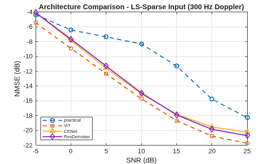
The results shown here use pretrained networks. The evaluation was run offline and saved to reduce example run time. The results use 500 slots per SNR point with TDL-C (300 ns delay spread, 300 Hz Doppler) and DMRSAdditionalPosition=1. The plot compares all three architectures trained with LS-sparse input against the nrChannelEstimate practical baseline. At 300 Hz Doppler, the practical estimator degrades significantly, and the neural networks provide 3 to 8 dB NMSE improvement at mid-to-high SNR.

testDoppler = 300;
allRes = load(fullfile("mimoceData",sprintf("eval_ls_sparse_mask_nmse_addpos1_dop%d.mat",testDoppler)));
res = allRes.results;
snrPts = res.snrPoints;

% Select methods for architecture comparison
archMethods = ["practical", "ViT", "CENet", "ResDenoiser"];
archIdx = ismember(res.methods, archMethods);
archNmse = res.allNmse(archIdx,:);
archNames = res.methods(archIdx);

figure
styles = {"--o", "--s", "-^", "-d", "-v"};
colors = lines(numel(archNames));
for m = 1:size(archNmse,1)
    plot(snrPts, archNmse(m,:), styles{m}, Color=colors(m,:), LineWidth=1.5)
    hold on
end
hold off
grid on
xlabel("SNR (dB)")
ylabel("NMSE (dB)")
title(sprintf("Architecture Comparison - LS-Sparse Input (%d Hz Doppler)",testDoppler))
legend(archNames, Location="southwest", FontSize=7)

Complexity Comparison

This table summarizes quality vs. complexity for each architecture using LS-sparse input. Full-band channel estimation (CE) cost assumes 13 PRGs per slot (52 RBs, 2x2 MIMO, 1 slot).

Architecture	Params	FLOPs per CE	Time per CE (CPU)	NMSE @ 25 dB	Tradeoffs
CENet	65K	115M	263 ms	-20.2 dB	Smallest; lightweight MLP-Mixer
ViT	182K	103M	608 ms	-21.7 dB	Best NMSE; slowest (attention overhead)
ResDenoiser	493K	8.5G	103 ms	-20.7 dB	Best speed due to optimized convolutions

ResDenoiser has the highest FLOPs (8.5G) yet the fastest wall-clock time (103 ms). Large-kernel convolutions are highly optimized on modern hardware (BLAS). ViT has 82x fewer FLOPs (103M) but is 6x slower (608 ms) due to dynamic tensor operations (reshape, permute) in self-attention that hinder compiler optimization. All architectures are bandwidth agnostic (PRG tiling), antenna-configuration agnostic (independent antenna-layer processing), and SNR adaptive.

NMSE Evaluation: Input Representation

This section keeps the architecture fixed to ViT and varies the input representation. The plot shows ViT NMSE for each input representation at 300 Hz Doppler with DMRSAdditionalPosition=1.

testDoppler = 300;
resPrac1 = load(fullfile("mimoceData",sprintf("eval_practical_nmse_addpos1_dop%d.mat",testDoppler)));
resInterp1 = load(fullfile("mimoceData",sprintf("eval_ls_interp_nmse_addpos1_dop%d.mat",testDoppler)));
resSparse1 = load(fullfile("mimoceData",sprintf("eval_ls_sparse_mask_nmse_addpos1_dop%d.mat",testDoppler)));
resCombined1 = buildInputComparisonStruct(resSparse1.results, resPrac1.results, resInterp1.results);
plotNMSEInputComparison(resCombined1,testDoppler);

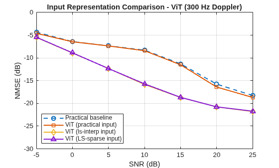
The practical-input ViT achieves performance close to the practical baseline because the nrChannelEstimate function have already smoothed the channel estimate before it is provided to the network. The LS-sparse and LS-interp ViTs achieve nearly identical NMSE because linear interpolation is a simple linear operation applied to the pilot observations. The ViT can learn this operation internally, so pre-computing the interpolation provides little benefit. The LS-sparse and LS-interp ViTs achieve lower NMSE than the practical-input ViT at all SNR values because they operate on raw pilot observations and allow the network to learn its own interpolation and denoising strategy.

Throughput Evaluation

NMSE measures estimation quality in isolation. To assess link-level impact, evaluate throughput using a full HARQ simulation with SVD precoding, LDPC coding, and 16-QAM modulation. The hEvaluateChannelEstimationThroughput helper function transmits precoded PDSCH through the channel, estimates the channel with each method, equalizes, decodes, and measures the block error rate (BLER) and throughput as a percentage of the peak rate.

% Load trained networks (LS-sparse input)
vit = load("trained_vit_ls_sparse_mask_addpos1.mat","trainedNet","networkMeta");
cenet = load("trained_cenet_ls_sparse_mask_addpos1.mat","trainedNet","networkMeta");
resden = load("trained_resden_ls_sparse_mask_addpos1.mat","trainedNet","networkMeta");

% Build estimator objects
estVit = hNNChannelEstimator(vit.trainedNet, vit.networkMeta);
estCENet = hNNChannelEstimator(cenet.trainedNet, cenet.networkMeta);
estResDen = hNNChannelEstimator(resden.trainedNet, resden.networkMeta);

% Evaluate throughput across SNR
results = hEvaluateChannelEstimationThroughput( ...
    {estVit, estCENet, estResDen}, ...
    MethodNames=["ViT","CENet","ResDenoiser"], ...
    DopplerHz=300, 
    DelaySpread_ns=300, 
    DelayProfile="TDL-C", ...
    NFrames=50, 
    SNRPoints=-5:5:25, ...
    Modulation="16QAM", 
    CodeRate=512/1024);

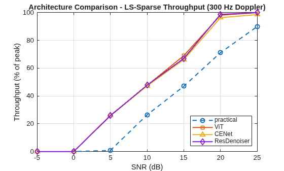
The results use pretrained networks with LS-sparse input, evaluated offline and are saved to reduce example run time. The channel conditions match the NMSE evaluation (TDL-C, 300 ns, 300 Hz Doppler, DMRSAdditionalPosition=1) with 16-QAM at rate 1/2 and 50 frames per SNR point. At 300 Hz Doppler, the practical estimator degrades significantly, while the neural network estimators with LS-sparse input maintain high throughput. To increase fidelity around the operating point, reduce the SNR range to the 70% to 100% throughput region and decrease the SNR step size.

testDoppler = 300;
tputData = load(fullfile("mimoceData",sprintf("eval_ls_sparse_mask_tput_addpos1_dop%d.mat",testDoppler)));
tputRes = tputData.results;

% Select methods for throughput comparison
archMethods = ["practical", "ViT", "CENet", "ResDenoiser"];
tputIdx = ismember(tputRes.methods, archMethods);
tputVals = tputRes.throughputPct(tputIdx,:);
tputNames = tputRes.methods(tputIdx);

figure
styles = {"--o", "-s", "-^", "-d", "-v"};
colors = lines(numel(tputNames));
for m = 1:size(tputVals,1)
    plot(tputRes.snrPoints, tputVals(m,:), styles{m}, Color=colors(m,:), LineWidth=1.5)
    hold on
end
hold off
grid on
xlabel("SNR (dB)")
ylabel("Throughput (% of peak)")
title(sprintf("Architecture Comparison - LS-Sparse Throughput (%d Hz Doppler)", testDoppler))
legend(tputNames, Location="southeast")

Summary

This example demonstrates how to build, train, and compare neural network channel estimators for 5G NR MIMO:

• Throughput gain scales with Doppler: At 300 Hz Doppler, all three NN architectures with LS-sparse input reach 98-100% throughput at 25 dB SNR, while the practical baseline saturates at 90%. The gain is 20-27 percentage points at mid-SNR (10-20 dB). At 10 Hz Doppler, the practical estimator already achieves 100% throughput at 20 dB and the NN contribution is limited to 6 percentage points at 15 dB. Architecture differences are small (within 3 percentage points), so architecture selection can be driven by complexity and latency constraints.

• Input representation matters: At 300 Hz Doppler, the LS-sparse input consistently outperforms the practical input across the entire SNR range. The practical estimator relies on CIR denoising and time interpolation, both of which introduce bias that the ViT cannot fully remove. In contrast, the LS-sparse input preserves the raw pilot observations, allowing the network to learn its own interpolation strategy. At lower Doppler frequencies (10-100 Hz), the two inputs perform similarly at low SNR, where CIR denoising and averaging effectively suppress noise. However, from approximately 5 dB SNR onward, the LS-sparse input begins to outperform the practical input, with the advantage becoming more pronounced at higher Doppler frequencies where the practical estimator's linear time interpolation reaches its limits.

• Modular workflow: The MATLAB implementation lets you change one variable at a time (architecture, input, Doppler, pilot density) and rerun the code to explore the design space.

Further Exploration

Extend the workflow to your scenario by modifying the channel and system parameters:

• Antenna configurations: 4x4, 8x2, or asymmetric arrays

• Higher-order modulation: 64-QAM and 256-QAM increase sensitivity to estimation errors

• Different delay profiles: TDL-A (LOS), TDL-D (rural), or CDL models for spatial consistency

• Additional conditioning: Extend FiLM to Doppler, delay spread, or other system parameters

NMSE improvements can translate to throughput gains at operating points where channel estimation error limits performance (for example, high modulation order or low-to-mid SNR). Use hEvaluateChannelEstimationThroughput to measure link-level impact for specific configurations.

Use hExploreChannelEstimationResults as an interactive results viewer to compare across architectures, input representations, and channel conditions. The function automatically discovers available evaluation data. When you run additional evaluations, the new configurations appear automatically.

hExploreChannelEstimationResults(DataFolder=dataFolder);

References

[1] E. Perez, F. Strub, H. de Vries, V. Dumoulin, and A. Courville, "FiLM: Visual Reasoning with a General Conditioning Layer," Proc. AAAI Conf. on Artificial Intelligence, 2018.

Helper Functions

This example uses the following helper files:

• hDeepLearningChanEstSimParameters — Default simulation parameters (2x2 MIMO, 52 RBs, 15 kHz SCS)

• hGenerate5GChannelEstimationData — Generate matched channel realizations in multiple input representations

• hPrepareChannelEstimationTrainingData — PRG tiling, real/imaginary split, RMS normalization for training

• hBuildChanEstViT — Build Vision Transformer architecture with FiLM conditioning

• hBuildChanEstCENet — Build MLP-Mixer (CENet) architecture with FiLM conditioning

• hBuildChanEstResDenoiser — Build residual denoiser CNN with FiLM conditioning

• hNNChannelEstimator — System object for inference (PRG tiling + SNR conditioning)

• hEvaluateChannelEstimationNMSE — Monte Carlo NMSE evaluation across SNR range

• hEvaluateChannelEstimationThroughput — Link-level throughput evaluation with HARQ and SVD precoding

• hExploreChannelEstimationResults — Interactive results viewer

• hLSChannelEstimate — LS estimation with CDM despreading and linear interpolation

• hGetDMRSConfig — DM-RS indices, symbols, and CDM lengths for a given comb factor

• hTrainChannelEstimationNetwork — Train a channel estimation network (ViT, CENet, or ResDenoiser)

• hReproduceAIMIMOChannelEstimationResults — Reproduce all shipped pretrained models and evaluation results

• hSlicePRGs / hAssemblePRGs — Slice and reassemble PRG sub-grids for bandwidth-agnostic processing

function plotChannelRepresentations(teaser)
prgIdx = 1:48;
fig = figure;
fig.Position(3) = fig.Position(3) * 2;
tiledlayout(1,4)
nexttile
vals = [abs(teaser.lsSparse(prgIdx,:,1,1)); abs(teaser.lsInterp(prgIdx,:,1,1)); ...
    abs(teaser.practical(prgIdx,:,1,1)); abs(teaser.perfect(prgIdx,:,1,1))];
colorLimits = [min(vals(:)), max(vals(:))];
imagesc(abs(teaser.lsSparse(prgIdx,:,1,1))); axis xy
clim(colorLimits)
title("Sparse (Pilots Only)"); xlabel("OFDM Symbol"); ylabel("Subcarrier")
nexttile
imagesc(abs(teaser.lsInterp(prgIdx,:,1,1))); axis xy
clim(colorLimits)
title("LS-Interp"); xlabel("OFDM Symbol"); ylabel("Subcarrier")
nexttile
imagesc(abs(teaser.practical(prgIdx,:,1,1))); axis xy
clim(colorLimits)
title("Practical"); xlabel("OFDM Symbol"); ylabel("Subcarrier")
nexttile
imagesc(abs(teaser.perfect(prgIdx,:,1,1))); axis xy
clim(colorLimits)
title("Perfect (Target)"); xlabel("OFDM Symbol"); ylabel("Subcarrier")
colorbar
end

function plotInference(inputEst4D,inputLabel,nnEst,architectureName,nmseNN,perfectEst4D)
prgIdx = 1:48;
fig = figure;
fig.Position(3) = fig.Position(3) * 1.5;
vals = [abs(inputEst4D(prgIdx,:,1,1)); abs(nnEst(prgIdx,:,1,1)); ...
    abs(perfectEst4D(prgIdx,:,1,1))];
colorLimits = [min(vals(:)), max(vals(:))];
tiledlayout(1,3)
sgtitle("Channel Magnitude |H| (first antenna-layer pair, first PRG)")
nexttile
imagesc(abs(squeeze(inputEst4D(:,:,1,1)))); 
axis xy
title(sprintf("%s Input", inputLabel))
xlabel("OFDM Symbol"); 
ylabel("Subcarrier"); 
clim(colorLimits)
nexttile
imagesc(abs(squeeze(nnEst(:,:,1,1)))); 
axis xy
title(sprintf("%s + %s\n(NMSE = %.1f dB)", architectureName, inputLabel, nmseNN))
xlabel("OFDM Symbol"); 
ylabel("Subcarrier");
clim(colorLimits)
nexttile
imagesc(abs(squeeze(perfectEst4D(:,:,1,1)))); 
axis xy
title("Perfect Channel")
xlabel("OFDM Symbol"); 
ylabel("Subcarrier"); 
clim(colorLimits)
colorbar
end

function plotNMSEInputComparison(res1, testDoppler)
% Compare ViT across input representations for AddPos=1.
snrPts = res1.snrPoints;
vitMethods = ["practical", "vit-practical", "vit-lsinterp", "vit-lssparse"];
vitLabels = ["Practical baseline", "ViT (practical input)", "ViT (ls-interp input)", "ViT (LS-sparse input)"];

figure
styles = {"--o", "-s", "-d", "-^"};
for k = 1:numel(vitMethods)
    idx = find(res1.methods == vitMethods(k), 1);
    if ~isempty(idx)
        plot(snrPts, res1.allNmse(idx,:), styles{k}, LineWidth=1.5)
        hold on
    end
end
ylim([-30 0])
hold off
grid on
xlabel("SNR (dB)")
ylabel("NMSE (dB)")
title(sprintf("Input Representation Comparison - ViT (%d Hz Doppler)", testDoppler))
legend(vitLabels, Location="southwest")
end

function combined = buildInputComparisonStruct(sparseRes, pracRes, interpRes)
% Combine per-input results into a struct with method names matching
% plotNMSEInputComparison expectations.
vitIdxSparse = find(sparseRes.methods == "ViT", 1);
vitIdxPrac = find(pracRes.methods == "ViT", 1);
vitIdxInterp = find(interpRes.methods == "ViT", 1);
pracIdx = find(sparseRes.methods == "practical", 1);
combined.snrPoints = sparseRes.snrPoints;
combined.methods = ["practical", "vit-practical", "vit-lsinterp", "vit-lssparse"];
combined.allNmse = [sparseRes.allNmse(pracIdx,:); ...
    pracRes.allNmse(vitIdxPrac,:); ...
    interpRes.allNmse(vitIdxInterp,:); ...
    sparseRes.allNmse(vitIdxSparse,:)];
end

function [pracData,interpData,sparseData,trainX,valX,nCh] = prepareData(numRealizations,snrRange,dopplerRange,delaySpreadRange,delayProfiles,simParameters,prgSizeRBs)
% Generate channel data and prepare three input representations for training.                        
%   Simulates numRealizations channel slots via hGenerate5GChannelEstimationData,
%   then calls hPrepareChannelEstimationTrainingData for each input type:
%   practical, LS-interp, and LS-sparse (with binary pilot mask).
%   Each representation undergoes: train/val split by realization, PRG tiling,
%   real/imaginary interleaving, and per-sample RMS normalization.

rawData = hGenerate5GChannelEstimationData(numRealizations, ...
    SNRRange=snrRange, DopplerRange=dopplerRange, ...
    DelaySpreadRange=delaySpreadRange, ...
    DelayProfiles=delayProfiles, ...
    SimParameters=simParameters, ...
    PrintProgress=true);
disp("Realizations: " + size(rawData.perfect, 4))

% Prepare three input representations for training. Each call applies the
% same preprocessing: train/val split by realization, antenna-layer
% processing, PRG extraction (4-RB sub-grids), real/imaginary
% interleaving, and per-sample RMS normalization.
pracData = hPrepareChannelEstimationTrainingData(rawData.practical, rawData.perfect, ...
    rawData.snrEstPractical, PRGSizeRBs=prgSizeRBs, SNRRange=snrRange);
pracData.dmrsSymIdx = rawData.dmrsSymIdx;
pracData.pilotMask = rawData.pilotMask;
interpData = hPrepareChannelEstimationTrainingData(rawData.lsInterp, rawData.perfect, ...
    rawData.snrEstInterp, PRGSizeRBs=prgSizeRBs, SNRRange=snrRange);
interpData.dmrsSymIdx = rawData.dmrsSymIdx;
interpData.pilotMask = rawData.pilotMask;
sparseData = hPrepareChannelEstimationTrainingData(rawData.lsSparse, rawData.perfect, ...
    rawData.snrEstSparse, PRGSizeRBs=prgSizeRBs, SNRRange=snrRange, ...
    MaskChannel=rawData.pilotMask);
sparseData.dmrsSymIdx = rawData.dmrsSymIdx;
sparseData.pilotMask = rawData.pilotMask;

trainX = pracData.trainX;
valX = pracData.valX;
nCh = pracData.nCh;
end