Test Automation from Simulation to Real-Time Testing
By Jon Lobo, MathWorks
As system designs grow more complex, so does the risk of relying on prototypes to determine whether the system performance meets the design requirement: the prototype can be costly, risky to operate, or even unavailable or incomplete by the time testing needs to start. As a result, more and more engineering teams are using simulation and other testing techniques early in the design process, when errors are easier and less costly to fix.
Simulink Test™ provides an integrated framework that lets you perform automated, repeatable tests throughout the design process, from desktop simulation to testing with hardware (Figure 1).

Figure 1. Framework for repeatable system testing through desktop and hardware-in-the-loop simulation.
To demonstrate this framework, we will use a flutter suppression example.
Flutter Suppression System Testing Goals and Setup
Flutter is the vibration caused by aerodynamic forces acting on an airplane wing. This phenomenon can have effects ranging from moderate turbulence to complete destruction of the wing. One way to control flutter is to use a control surface and attempt to dampen the vibration.
Our flutter suppression system takes three inputs: desired angle (in degrees), speed (in Mach), and altitude (in feet). Its single output is the measured deflection of the wing (in radians).
We want to test the system against two design requirements:
- The system suppresses flutter to within 0.005 radians within two seconds of a disturbance being applied.
- Flutter decays exponentially over time—specifically, the system has a positive damping ratio.
The system will need to meet these requirements under a variety of operating conditions to minimize unexpected behavior when it’s deployed in the field or put into production.
Figure 2 shows the Simulink® model of our flutter suppression system.

Figure 2. Aircraft flutter suppression system model.
In this model, we will introduce a disturbance after three seconds and then test whether the controller can dampen flutter at a variety of Mach and altitude points. To perform these tests, we will need the following:
- A testing environment that can monitor the flutter at each time step of the simulation
- The ability to log data to determine whether the flutter has decayed exponentially over time
- The ability to iterate over various values for Mach and altitude
Setting Up a Test Harness Test Sequence Block
Control design engineers sometimes create two separate models, one for testing and another for implementation. Making sure that the base model and the implemented model remain equivalent can be challenging. Additionally, depending on the testing task, it might be necessary to customize inputs or log additional data, which will change the base model.
Simulink provides two tools that enable us to avoid this version control issue: a test harness and a Test Sequence block. The test harness is a model block diagram that is associated with a component of the system under test. It contains a separate model workspace and configuration set, yet it persists within the main model. It effectively gives us a sandbox to test our design without changing or corrupting the base model.
To create a test harness from scratch in Simulink, we simply right-click on a subsystem or select Analysis from the toolstrip and select Test Harness followed by Create Test Harness. We can then configure the new test harness interactively (Figure 3).
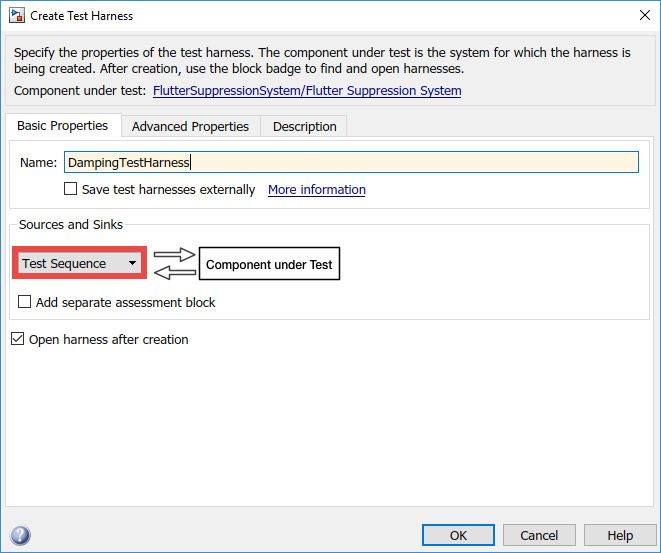
Figure 3. Test harness dialog box in Simulink.
The Test Sequence block (shown in red in Figure 4) uses MATLAB® as an action language (Figure 5). It allows you to transition between test steps conditionally while evaluating a component under test. You can use conditional logic, temporal operators (such as before and after), and event operators, such as hasChanged and hasChangedFrom.

Figure 4. Test harness model with Test Sequence block (red) and data logging (blue).

Figure 5. Test sequence with MATLAB action language.
The first requirement dictates that the flutter shall be bounded within two seconds of the initial disturbance being applied. We incorporate a Test Sequence block to implement this test case. We set the desired position to 0 radians, and after five seconds, calculate the error at each time step. The verify function allows us to log whether this condition was met at each time step.
To calculate the damping ratio, we will log data both in simulation and in real time through the To Workspace and File Scope blocks indicated in blue in Figure 4.
Creating and Running Desktop Simulations
The system under test has two inputs: Mach and altitude. The requirements specify that the system should be tested under a variety of operating conditions. We can vary the conditions by using the Simulink Test Manager to create an automated test suite. The test suite will enable us to automatically test both requirements over varying input conditions and generate reports on whether they pass or fail. This test suite can be rerun as the design changes.
Using the Test Manager, we create a new simulation test for the flutter suppression system, add a description to identify the purpose of the test, and link it to the requirements. Finally, we specify some operating conditions for Mach and altitude using scripted iterations (Figure 6).
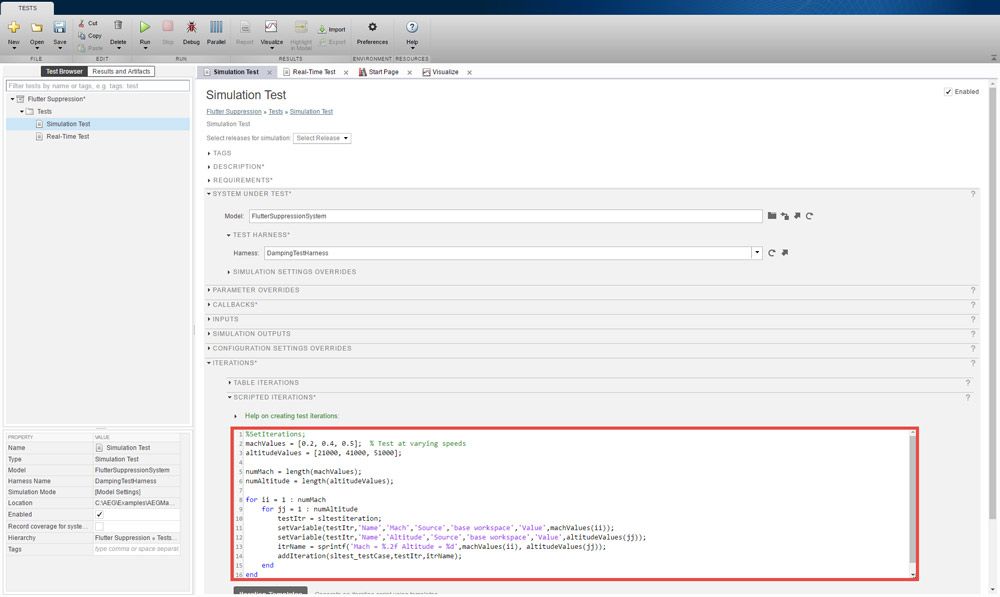
Figure 6. Setting iterations for different Mach and altitude values using a MATLAB script in the Test Manager interface.
We will now use this test automation workflow to test our two requirements. The first requirement was handled with the Test Sequence block. Recall the use of the verify function. If at any point the verify criteria fail, the overall test will fail.
For the second requirement, we added blocks to log simulation data. We need to do some data analysis on the measured angle to determine whether the test has passed or failed. This analysis can be done through the cleanup callback that executes after each simulation run (Figure 7). We can leverage previous data analysis work to do an exponential fit and declare pass or fail based on the fit parameters.
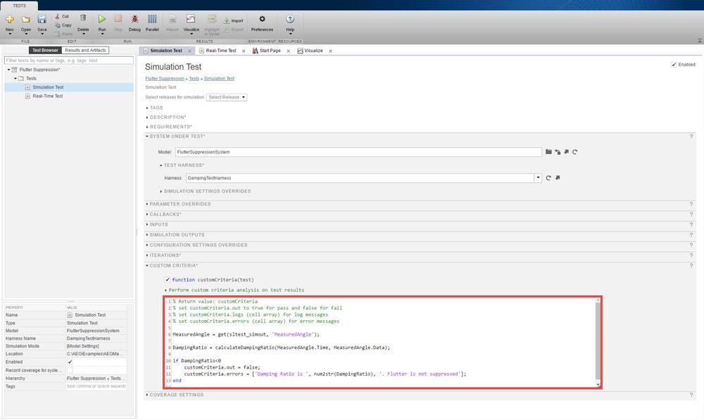
Figure 7. Setting up the cleanup callback for custom criteria in the Test Manager interface.
From here, this test will automatically exercise our system with the operating conditions we have specified. We can see the test results in the Results and Artifacts pane (Figure 8). We can check the output of the verify statement and identify times when the test criteria were not evaluated, when it passed, and when it failed. Additionally, we can visualize the logged Commanded and Measured Angle data.
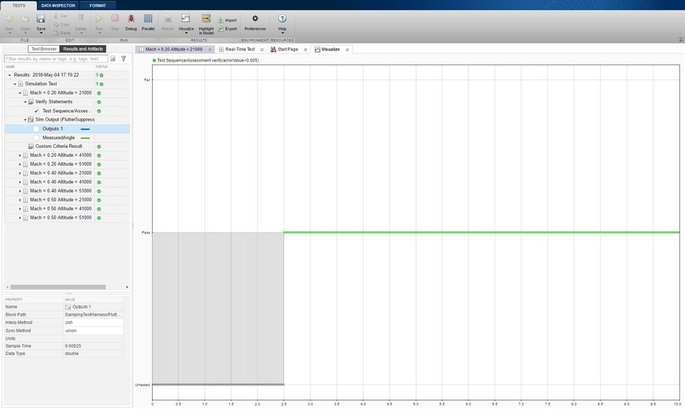
Figure 8. Output of verify statement (requirement 1).
The system passed all the tests in simulation, but let’s take a closer look to make sure the requirements have been met. Recall the requirement that the flutter shall be bounded within two seconds of a disturbance being applied. Given that the disturbance is applied three seconds into the simulation, it is expected that the verify statement is untested for the first five seconds of simulation. From there on we can see that the test passed.
The measured angle data shows that the flutter is not only bounded but also decaying, which fulfills the second requirement (Figure 9).

Figure 9. Measured angle output.
Real-Time Testing
We’re now ready to test with hardware using hardware-in-the-loop (HIL) simulation. The goal of HIL is to simulate the plant model dynamics in real time while interfacing with the embedded controller that will be used in the field. For HIL we’ll be using a laptop computer running Simulink, a Speedgoat real-time target, and an embedded controller connected through analog and discrete I/O (Figure 10).

Figure 10. Test hardware: Windows PC (red), Speedgoat target (blue), and embedded controller (green).
On the laptop, we generate C code from the model and compile it to a real-time application, which is downloaded to the Speedgoat real-time target computer over an Ethernet connection. The generated code includes the plant model dynamics, the drivers for the I/O required to communicate with the controller, and the test assessment block containing the verify function.
A key difference between the simulation and real-time tests is that we remove the simulated control system and use the control system implemented on the embedded processor. We can then test the implemented control system with its field inputs and outputs at its natural operating frequency.
We’ll now use the Test Manager to create a real-time test (Figure 11).

Figure 11. Test Manager interface for setting up a real-time test.
In the real-time test we populate the same fields as before, plus an additional field for the system under test, Target Computer. This field can be used to specify the real-time target computer that the test will run on.
We will test the requirements under the same varying operating conditions as before, and we’ll do the same data analysis on the measured angle to determine whether the test has passed or failed. We can view the results in the Test Manager (Figure 12).

Figure 12. Real-time test results.
We find that the real-time test fails for some of the test conditions. As Figure 12 and Figure 13 show, the verify statement fails at various points and the measured angle does not decay, resulting in an unstable system.

Figure 13. Measured angle output from real-time test.
What was different about this test that caused it fail when it passed in simulation?
There are several reasons why these tests failed, and these reasons highlight the importance of testing with hardware. First, in the simulation model, the controller and plant were directly connected using double-precision values as the interface. The connection between the real-time simulation and the production controller is through digital and analog signals, and so right away we lose precision, due to quantization, in the interface. Second, the simulation testing did not account for the real-world latencies that exist in actual systems. Third, it is possible that the control design that was tested in simulation was not implemented correctly in the production controller.
Even though these tests did not pass and we still have work to do, we want to create a report to send to colleagues. Using the report generator from within the Test Manager, we create a report that documents who performed the tests, the test criteria, the links to the requirements, and a summary of the results.
As the system design evolves, we can use the Test Manager and the tests we have already created to automatically perform regression tests and generate the reports for those, as well.
Benefits of Test Automation
This article demonstrated a framework for testing systems against requirements throughout the design process. Using Simulink Test, we were able to create repeatable tests that verify our requirements in two different ways: one with the test criteria in the control loop and another with more conventional postprocessing. We could link the tests to the design requirements to ensure traceability and automatically test the requirements against a variety of inputs.
As the test results demonstrated, simulation and real-world behavior do not always match—hence the need to test designs early and with the same interfaces used in the field. Lastly, we can use Simulink Real-Time™ with Simulink Test to create real-time tests that verify the design without the real-world system or the risk of damaging a prototype.
Published 2018