Main Content

uss

Uncertain state-space model

Description

Use uss model objects to represent uncertain dynamic systems.

The two dominant forms of model uncertainty are:

  • Uncertainty in parameters of the underlying differential equation models (uncertain state-space matrices)

  • Frequency-domain uncertainty, which often quantifies model uncertainty by describing absolute or relative uncertainty in the frequency response (uncertain or unmodeled linear dynamics)

uss model objects can represent dynamic systems with either or both forms of uncertainty. You can use uss to perform robust stability and performance analysis and to test the robustness of controller designs.

Creation

There are several ways to create a uss model object, including:

  • Use tf with one or more uncertain real parameters (ureal). For example:

    p = ureal('p',1);
    usys = tf(p,[1 p]);

    For another example, see Transfer Function with Uncertain Coefficients.

  • Use ss with uncertain state-space matrices (umat). For example:

    p = ureal('p',1);
    A = [0 3*p; -p p^2];
    B = [0; p];
    C = ones(2);  
    D = zeros(2,1);
    usys = ss(A,B,C,D);

    For another example, see Uncertain State-Space Model.

  • Combine numeric LTI models with uncertain elements using model interconnection commands such as connect, series, or parallel, or model arithmetic operators such as *, +, or -. For example:

     sys = tf(1,[1 1]);
     p = ureal('p',1);
     D = ultidyn('Delta',[1 1]);
     usys = p*sys*(1 + 0.1*D);

    For another example, see System with Uncertain Dynamics.

  • Convert a double array or a numeric LTI model to uss form using usys = uss(sys). In this case, the resulting uss model object has no uncertain elements. For example:

    M = tf(1,[1 1 1]);
    usys = uss(M);
  • Use ucover to create a uss model whose range of possible frequency responses includes all responses in an array of numeric LTI models. The resulting model expresses the range of behaviors as dynamic uncertainty (ultidyn).

Properties

expand all

Nominal value of the uncertain model, specified as a state-space (ss) model object. The state-space model is obtained by setting all the uncertain control design blocks of the uncertain model to their nominal values.

Uncertain elements of the model, specified as a structure whose fields are the names of the uncertain blocks, and whose values are the control design blocks themselves. Thus, the values stored in the structure can be ureal, umat, ultidyn, or other uncertain control design blocks. For instance, the following commands create an uncertain model usys with two uncertain parameters, p1 and p2.

p1 = ureal('p1',1);
p2 = ureal('p2',3);
A = [0 3*p1; -p1 p1^2];
B = [0; p2];
C = ones(2);
D = zeros(2,1);
usys = ss(A,B,C,D);

The Uncertainty property of usys is a structure with two fields, p1 and p2, whose values are the corresponding ureal uncertain parameters.

usys.Uncertainty
ans = 

  struct with fields:

    p1: [1×1 ureal]
    p2: [1×1 ureal]

You can access or examine each uncertain parameter individually. For example:

get(usys.Uncertainty.p1)
    NominalValue: 1
            Mode: 'PlusMinus'
           Range: [0 2]
       PlusMinus: [-1 1]
      Percentage: [-100 100]
    AutoSimplify: 'basic'
            Name: 'p1'

This property is read-only.

State-space matrices, specified as numeric matrices or uncertain matrices (umat). The state-space matrices are evaluated by fixing all dynamic uncertainty blocks (udyn, ultidyn) to their nominal values.

  • A — State matrix A, specified as a square matrix or umat with as many rows and columns as there are system states.

  • B — Input-to-state matrix B, specified as a matrix or umat with as many rows as there are system states and as many columns as there are system inputs.

  • C — State-to-output matrix C, specified as a matrix or umat with as many rows as there are system outputs and as many columns as there are system states.

  • D — Feedthrough matrix D, specified as a matrix or umat with as many rows as there are system outputs and as many columns as there are system inputs.

  • EE matrix for implicit (descriptor) state-space models, specified as a matrix or umat of the same dimensions as A. By default E = [], meaning that the state equation is explicit. To specify an implicit state equation E dx/dt = Ax + Bu, set this property to a square matrix of the same size as A. See dss for more information about descriptor state-space models.

State names, specified as:

  • A character vector or string — For first-order models

  • A cell array of character vectors or string array — For models with two or more states

  • '' — For unnamed states

If you specify StateName using a string, such as "velocity", the state name is stored as a character vector, 'velocity'.

Example: 'velocity'

Example: {'x1','x2'}

State units, specified as:

  • A character vector or string — For first-order models

  • A cell array of character vectors or string array — For models with two or more states

  • '' — For states without specified units

Use StateUnit to keep track of the units each state is expressed in. StateUnit has no effect on system behavior.

If you specify StateUnit using a string, such as "mph", the state units are stored as a character vector, 'mph'.

Example: 'mph'

Example: {'rpm','rad/s'}

Internal delays, specified as a scalar or vector. For continuous-time models, internal delays are expressed in the time unit specified by the TimeUnit property of the model object. For discrete-time models, internal delays are expressed as integer multiples of the sample time Ts. For example, InternalDelay = 3 means a delay of three sampling periods.

You can modify the values of internal delays. However, the number of entries in InternalDelay cannot change, because it is a structural property of the model.

Internal delays arise, for example, when closing feedback loops on systems with delays, or when connecting delayed systems in series or parallel. For more information about internal delays, see Closing Feedback Loops with Time Delays.

Delay at each input, specified as a scalar or a vector. For a system with Nu inputs, set InputDelay to an Nu-by-1 vector. Each entry of this vector is a numerical value that represents the input delay for the corresponding input channel. For continuous-time models, specify input delays in the time unit stored in the TimeUnit property of the model object. For discrete-time models, specify input delays in integer multiples of the sample time Ts. For example, InputDelay = 3 means a delay of three sample times.

Set InputDelay to a scalar value to apply the same delay to all channels.

Delay at each output, specified as a scalar or a vector. For a system with Ny outputs, set OutputDelay to an Ny-by-1 vector. Each entry of this vector is a numerical value that represents the output delay for the corresponding output channel. For continuous-time models, specify output delays in the time unit stored in the TimeUnit property of the model object. For discrete-time models, specify output delays in integer multiples of the sample time Ts. For example, OutputDelay = 3 means a delay of three sample times.

Set OutputDelay to a scalar value to apply the same delay to all channels.

Sample time, specified as:

  • 0 — For continuous-time models.

  • Positive scalar value — For discrete-time models. Specify the sample time in the units given in the TimeUnit property of the model.

  • –1 — For discrete-time models with unspecified sample time.

Changing this property does not discretize or resample the model.

Model time units, specified as:

  • 'nanoseconds'

  • 'microseconds'

  • 'milliseconds'

  • 'seconds'

  • 'minutes'

  • 'hours'

  • 'days'

  • 'weeks'

  • 'months'

  • 'years'

If you specify TimeUnit using a string, such as "hours", the time units are stored as a character vector, 'hours'.

Model properties such as sample time Ts, InputDelay, OutputDelay, and other time delays are expressed in the units specified by TimeUnit. Changing this property has no effect on other properties, and therefore changes the overall system behavior. Use to convert between time units without modifying system behavior.

Names of input channels, specified as:

  • A character vector or string — For single-input models

  • A cell array of character vectors or a string array — For models with two or more inputs

  • '' — For inputs without specified names

You can use automatic vector expansion to assign input names for multi-input models. For example, if sys is a two-input model, you can specify InputName as follows.

sys.InputName = 'controls';

The input names automatically expand to {'controls(1)';'controls(2)'}.

You can use the shorthand notation u to refer to the InputName property. For example, sys.u is equivalent to sys.InputName.

Input channel names have several uses, including:

  • Identifying channels on model display and plots

  • Extracting subsystems of MIMO systems

  • Specifying connection points when interconnecting models

If you specify InputName using a string or string array, such as "voltage", the input name is stored as a character vector, 'voltage'.

Units of input signals, specified as:

  • A character vector or string — For single-input models

  • A cell array of character vectors or string array — For models with two or more inputs

  • '' — For inputs without specified units

Use InputUnit to keep track of the units each input signal is expressed in. InputUnit has no effect on system behavior.

If you specify InputUnit using a string, such as "voltage", the input units are stored as a character vector, 'voltage'.

Example: 'voltage'

Example: {'voltage','rpm'}

Input channel groups, specified as a structure where the fields are the group names and the values are the indices of the input channels belonging to the corresponding group. When you use InputGroup to assign the input channels of MIMO systems to groups, you can refer to each group by name when you need to access it. For example, suppose you have a five-input model sys, where the first three inputs are control inputs and the remaining two inputs represent noise. Assign the control and noise inputs of sys to separate groups.

sys.InputGroup.controls = [1:3];
sys.InputGroup.noise = [4 5];

Use the group name to extract the subsystem from the control inputs to all outputs.

sys(:,'controls')

Example: struct('controls',[1:3],'noise',[4 5])

Names of output channels, specified as:

  • A character vector or string— For single-output models

  • A cell array of character vectors or string array — For models with two or more outputs

  • '' — For outputs without specified names

You can use automatic vector expansion to assign output names for multi-output models. For example, if sys is a two-output model, you can specify OutputName as follows.

sys.OutputName = 'measurements';

The output names automatically expand to {'measurements(1)';'measurements(2)'}.

You can use the shorthand notation y to refer to the OutputName property. For example, sys.y is equivalent to sys.OutputName.

Output channel names have several uses, including:

  • Identifying channels on model display and plots

  • Extracting subsystems of MIMO systems

  • Specifying connection points when interconnecting models

If you specify OutputName using a string, such as "rpm", the output name is stored as a character vector, 'rpm'.

Units of output signals, specified as:

  • A character vector or string — For single-output models

  • A cell array of character vectors or string array — For models with two or more outputs

  • '' — For outputs without specified units

Use OutputUnit to keep track of the units each output signal is expressed in. OutputUnit has no effect on system behavior.

If you specify OutputUnit using a string, such as "voltage", the output units are stored as a character vector, 'voltage'.

Example: 'voltage'

Example: {'voltage','rpm'}

Output channel groups, specified as a structure where the fields are the group names and the values are the indices of the output channels belonging to the corresponding group. When you use OutputGroup to assign the output channels of MIMO systems to groups, you can refer to each group by name when you need to access it. For example, suppose you have a four-output model sys, where the second output is a temperature, and the rest are state measurements. Assign these outputs to separate groups.

sys.OutputGroup.temperature = [2];
sys.OutputGroup.measurements = [1 3 4];

Use the group name to extract the subsystem from all inputs to the measurement outputs.

sys('measurements',:)

Example: struct('temperature',[2],'measurement',[1 3 4])

Text notes about the model, specified as a string or character vector. The property stores whichever of these two data types you provide. For instance, suppose that sys1 and sys2 are dynamic system models. You can set their Notes properties to a string and a character vector, respectively.

sys1.Notes = "sys1 has a string.";
sys2.Notes = 'sys2 has a character vector.';
sys1.Notes
sys2.Notes
ans = 

    "sys1 has a string."


ans =

    'sys2 has a character vector.'

You can also specify Notes as string array or a cell array of character vectors or strings.

Data of any kind that you want to associate and store with the model, specified as any MATLAB® data type.

Model name, stored as a character vector or string. If you specify Name using a string, such as "DCmotor", the string is stored as a character vector, 'DCmotor'.

Example: 'system_1'

Sampling grid for model arrays, specified as a structure. For model arrays that are derived by sampling one or more independent variables, this property tracks the variable values associated with each model in the array. This information appears when you display or plot the model array. Use this information to trace results back to the independent variables.

Set the field names of the data structure to the names of the sampling variables. Set the field values to the sampled variable values associated with each model in the array. All sampling variables should be numeric and scalar valued, and all arrays of sampled values should match the dimensions of the model array.

For example, suppose you create a 11-by-1 array of linear models, sysarr, by taking snapshots of a linear time-varying system at times t = 0:10. The following code stores the time samples with the linear models.

 sysarr.SamplingGrid = struct('time',0:10)

Similarly, suppose you create a 6-by-9 model array, M, by independently sampling two variables, zeta and w. The following code attaches the (zeta,w) values to M.

[zeta,w] = ndgrid(<6 values of zeta>,<9 values of w>)
M.SamplingGrid = struct('zeta',zeta,'w',w)

When you display M, each entry in the array includes the corresponding zeta and w values.

M
M(:,:,1,1) [zeta=0.3, w=5] =
 
        25
  --------------
  s^2 + 3 s + 25
 

M(:,:,2,1) [zeta=0.35, w=5] =
 
         25
  ----------------
  s^2 + 3.5 s + 25
 
...

For model arrays generated by linearizing a Simulink® model at multiple parameter values or operating points, the software populates SamplingGrid automatically with the variable values that correspond to each entry in the array. For example, the Simulink Control Design™ commands linearize (Simulink Control Design) and slLinearizer (Simulink Control Design) populate SamplingGrid in this way.

Object Functions

Most functions that work on numeric LTI models also work on uss models. These include model interconnection functions such as connect and feedback, and linear analysis functions such as bode and stepinfo. Some functions that generate plots, such as bode and step, plot random samples of the uncertain model to give you a sense of the distribution of uncertain dynamics. When you use these commands to return data, however, they operate on the nominal value of the system only.

In addition, you can use functions such as robstab and wcgain to perform robustness and worst-case analysis of uncertain systems represented by uss models. You can also use tuning functions such as systune for robust controller tuning.

The following lists contain a representative subset of the functions you can use with uss models.

expand all

feedbackFeedback connection of multiple models
connectBlock diagram interconnections of dynamic systems
seriesSeries connection of two models
parallelParallel connection of two models
stepStep response of dynamic system
bodeBode plot of frequency response, or magnitude and phase data
sigmaSingular value plot of dynamic system
marginGain margin, phase margin, and crossover frequencies
diskmarginDisk-based stability margins of feedback loops
usampleGenerate random samples of uncertain model or element
robstabRobust stability of uncertain system
robgainRobust performance of uncertain system
wcgainWorst-case gain of uncertain system
wcsigmaplotPlot worst-case gain of uncertain system
musynRobust controller design using mu synthesis
systuneTune fixed-structure control systems modeled in MATLAB

Examples

collapse all

Create a second-order transfer function with uncertain natural frequency and damping coefficient.

w0 = ureal('w0',10);
zeta = ureal('zeta',0.7,'Range',[0.6,0.8]);

usys = tf(w0^2,[1 2*zeta*w0 w0^2])
Uncertain continuous-time state-space model with 1 outputs, 1 inputs, 2 states.
The model uncertainty consists of the following blocks:
  w0: Uncertain real, nominal = 10, variability = [-1,1], 5 occurrences
  zeta: Uncertain real, nominal = 0.7, range = [0.6,0.8], 1 occurrences

Type "usys.NominalValue" to see the nominal value and "usys.Uncertainty" to interact with the uncertain elements.

usys is an uncertain state-space (uss) model with two Control Design Blocks. The uncertain real parameter w0 occurs five times in the transfer function, twice in the numerator and three times in the denominator. To reduce the number of occurrences, you can rewrite the transfer function by dividing numerator and denominator by w0^2.

usys = tf(1,[1/w0^2 2*zeta/w0 1])
Uncertain continuous-time state-space model with 1 outputs, 1 inputs, 2 states.
The model uncertainty consists of the following blocks:
  w0: Uncertain real, nominal = 10, variability = [-1,1], 3 occurrences
  zeta: Uncertain real, nominal = 0.7, range = [0.6,0.8], 1 occurrences

Type "usys.NominalValue" to see the nominal value and "usys.Uncertainty" to interact with the uncertain elements.

In the new formulation, there are only three occurrences of the uncertain parameter w0. Reducing the number of occurrences of a Control Design Block in a model can improve the performance of calculations involving the model.

Examine the step response of the system to get a sense of the range of responses that the uncertainty represents.

step(usys)

Figure contains an axes object. The axes object contains 21 objects of type line. This object represents usys.

When you use linear analysis commands like step and bode to create response plots of uncertain systems, they automatically plot random samples of the system. While these samples give you a sense of the range of responses that fall within the uncertainty, they do not necessarily include the worst-case response. To analyze worst-case responses of uncertain systems, use wcgain or wcsigmaplot.

To create an uncertain state-space model, you first use Control Design Blocks to create uncertain elements. Then, use the elements to specify the state-space matrices of the system.

For instance, create three uncertain real parameters and build state-spaces matrices from them.

p1 = ureal('p1',10,'Percentage',50); 
p2 = ureal('p2',3,'PlusMinus',[-.5 1.2]); 
p3 = ureal('p3',0); 

A = [-p1 p2; 0 -p1]; 
B = [-p2; p2+p3]; 
C = [1 0; 1 1-p3]; 
D = [0; 0];

The matrices constructed with uncertain parameters, A, B, and C, are uncertain matrix (umat) objects. Using them as inputs to ss results in a 2-output, 1-input, 2-state uncertain system.

sys = ss(A,B,C,D)
Uncertain continuous-time state-space model with 2 outputs, 1 inputs, 2 states.
The model uncertainty consists of the following blocks:
  p1: Uncertain real, nominal = 10, variability = [-50,50]%, 2 occurrences
  p2: Uncertain real, nominal = 3, variability = [-0.5,1.2], 2 occurrences
  p3: Uncertain real, nominal = 0, variability = [-1,1], 2 occurrences

Type "sys.NominalValue" to see the nominal value and "sys.Uncertainty" to interact with the uncertain elements.

The display shows that the system includes the three uncertain parameters.

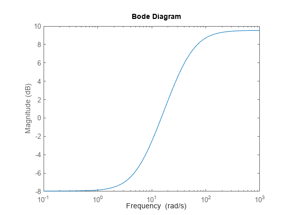
Create an uncertain system comprising a nominal model with a frequency-dependent amount of uncertainty. You can model such uncertainty using ultidyn and a weighting function that represents the frequency profile of the uncertainty. Suppose that at low frequency, below 3 rad/s, the model can vary up to 40% from its nominal value. Around 3 rad/s, the percentage variation starts to increase. The uncertainty crosses 100% at 15 rad/s and reaches 2000% at approximately 1000 rad/s. Create a transfer function with an appropriate frequency profile, Wunc, to use as a weighting function that modulates the amount of uncertainty with frequency.

Wunc = makeweight(0.40,15,3);
bodemag(Wunc)

Figure contains an axes object. The axes object with ylabel Magnitude (dB) contains an object of type line. This object represents Wunc.

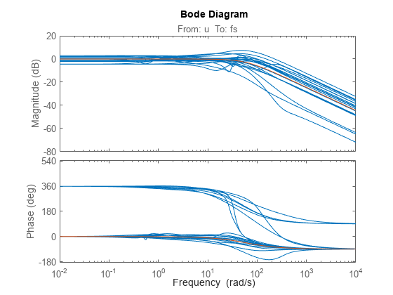
Next, create a transfer function representing the nominal value of the system. For this example, use a transfer function with a single pole at s = –60 rad/s. Then, create a ultidyn model to represent 1-input, 1-output uncertain dynamics, and add the weighted uncertainty to the nominal transfer function.

sysNom = tf(1,[1/60 1]);
unc = ultidyn('unc',[1 1],'SampleStateDim',3); % samples of uncertain dynamics have three states

usys = sysNom*(1 + Wunc*unc);

% Set properties of usys
usys.InputName = 'u';
usys.OutputName = 'fs';

Examine random samples of usys to see the effect of the uncertain dynamics.

bode(usys,usys.Nominal)

Figure contains 2 axes objects. Axes object 1 with title From: u To: fs, ylabel Magnitude (dB) contains 22 objects of type line. These objects represent usys, untitled1. Axes object 2 with ylabel Phase (deg) contains 22 objects of type line. These objects represent usys, untitled1.

uss models, like all model objects, include properties that store dynamics and model metadata. View the properties of an uncertain state-space model.

p1 = ureal('p1',10,'Percentage',50);
p2 = ureal('p2',3,'PlusMinus',[-.5 1.2]);
p3 = ureal('p3',0);
A = [-p1 p2; 0 -p1];
B = [-p2; p2+p3];
C = [1 0; 1 1-p3];
D = [0; 0];
sys = ss(A,B,C,D);     % create uss model

get(sys)
     NominalValue: [2x1 ss]
      Uncertainty: [1x1 struct]
                A: [2x2 umat]
                B: [2x1 umat]
                C: [2x2 umat]
                D: [2x1 double]
                E: []
        StateName: {2x1 cell}
        StateUnit: {2x1 cell}
    InternalDelay: [0x1 double]
       InputDelay: 0
      OutputDelay: [2x1 double]
        InputName: {''}
        InputUnit: {''}
       InputGroup: [1x1 struct]
       OutputName: {2x1 cell}
       OutputUnit: {2x1 cell}
      OutputGroup: [1x1 struct]
            Notes: [0x1 string]
         UserData: []
             Name: ''
               Ts: 0
         TimeUnit: 'seconds'
     SamplingGrid: [1x1 struct]

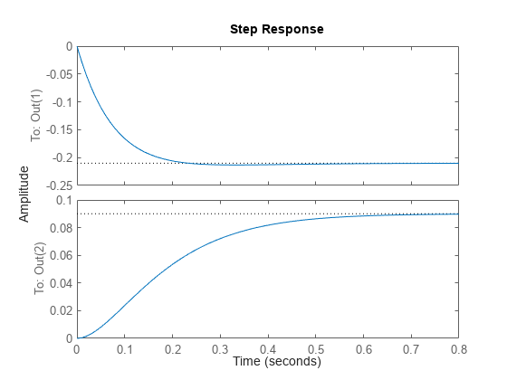
Most of the properties behave similarly to how they behave for ss model objects. The NominalValue property is itself an ss model object. You can therefore analyze the nominal value as you would any state-space model. For instance, compute the poles and step response of the nominal system.

pole(sys.NominalValue)
ans = 2×1

   -10
   -10

step(sys.NominalValue)

Figure contains 2 axes objects. Axes object 1 with ylabel To: Out(1) contains an object of type line. This object represents untitled1. Axes object 2 with ylabel To: Out(2) contains an object of type line. This object represents untitled1.

As with the uncertain matrices (umat), the Uncertainty property is a structure containing the uncertain elements. You can use this property for direct access to the uncertain elements. For instance, check the Range of the uncertain element named p2 within sys.

sys.Uncertainty.p2.Range
ans = 1×2

    2.5000    4.2000

Change the uncertainty range of p2 within sys.

sys.Uncertainty.p2.Range = [2 4];

This command changes only the range of the parameter called p2 in sys. It does not change the variable p2 in the MATLAB workspace.

p2.Range
ans = 1×2

    2.5000    4.2000

Version History

Introduced before R2006a